04
-
- 4.1 Introduction
- This section discusses the analysis of fluid in motion - fluid dynamics.
The motion of fluids can be predicted in the same way as the motion of solids are predicted using the fundamental laws of physics together with the physical properties of the fluid. It is not difficult to envisage a very complex fluid flow. Spray behind a car; waves on beaches; hurricanes and tornadoes or any other atmospheric phenomenon are all example of highly complex fluid flows which can be analysed with varying degrees of success (in some cases hardly at all!). However, there are many common situations which are easily analysed. -
- 4.2 Objectives
- ● Introduce concepts necessary to analyse fluids in motion
● Identify differences between Steady/unsteady uniform/non-uniform and compressible/incompressible flow
● Demonstrate streamlines and stream tubes
● Introduce the Continuity principle
● Demonstrate practical uses of the continuity equation in the analysis of flow
-
- 4.3 Uniform Flow, Steady Flow
- It is possible - and useful - to classify the type of flow which is being examined into small number of groups. If we look at a fluid flowing under normal circumstances - a river for example - the conditions at one point will vary from those at another point (e.g. different velocity) we have non-uniform flow. If the conditions at one point vary as time passes then we have unsteady flow. Under some circumstances the flow will not be as changeable as this. The following terms describe the states which are used to classify fluid flow:
● uniform flow: If the flow velocity is the same magnitude and direction at every point in the fluid it is said to be uniform.
● non-uniform: If at a given instant, the velocity is not the same at every point the flow is non-uniform. (In practice, by this definition, every fluid that flows near a solid boundary will be non-uniform – as the fluid at the boundary must take the speed of the boundary, usually zero. However if the size and shape of the of the cross-section of the stream of fluid is constant the flow is considered uniform.)
● steady: A steady flow is one in which the conditions (velocity, pressure and cross-section) may differ from point to point but DO NOT change with time.
● unsteady: If at any point in the fluid, the conditions change with time, the flow is described as unsteady. (In practise there are always slight variations in velocity and pressure, but if the average values are constant, the flow is considered steady.
Combining the above we can classify any flow in to one of four type:
1. Steady uniform flow. Conditions do not change with position in the stream or with time. An example is the flow of water in a pipe of constant diameter at constant velocity.
2. Steady non-uniform flow. Conditions change from point to point in the stream but do not change with time. An example is flow in a tapering pipe with constant velocity at the inlet - velocity will change as you move along the length of the pipe toward the exit.
3. Unsteady uniform flow. At a given instant in time the conditions at every point are the same, but will change with time. An example is a pipe of constant diameter connected to a pump pumping at a constant rate which is then switched off.
4. Unsteady non-uniform flow. Every condition of the flow may change from point to point and with time at every point. For example waves in a channel.
- If you imaging the flow in each of the above classes you may imagine that one class is more complex than another. And this is the case - steady uniform flow is by far the most simple of the four. You will then be pleased to hear that this course is restricted to only this class of flow. We will not be encountering any non-uniform or unsteady effects in any of the examples (except for one or two quasi-time dependent problems which can be treated at steady).
4.3.1 Compressible or Incompressible
All fluids are compressible - even water - their density will change as pressure changes. Under steady conditions, and provided that the changes in pressure are small, it is usually possible to simplify analysis of the flow by assuming it is incompressible and has constant density. As you will appreciate, liquids are quite difficult to compress - so under most steady conditions they are treated as incompressible. In some unsteady conditions very high pressure differences can occur and it is necessary to take these into account - even for liquids. Gasses, on the contrary, are very easily compressed, it is essential in most cases to treat these as compressible, taking changes in pressure into account.
4.3.2 Three-dimensional flow
Although in general all fluids flow three-dimensionally, with pressures and velocities and other flow properties varying in all directions, in many cases the greatest changes only occur in two directions or even only in one. In these cases changes in the other direction can be effectively ignored making analysis much more simple.
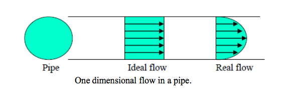
Flow is one dimensional if the flow parameters (such as velocity, pressure, depth etc.) at a given instant in time only vary in the direction of flow and not across the cross- section. The flow may be unsteady, in this case the parameter vary in time but still not across the cross-section. An example of one-dimensional flow is the flow in a pipe.
Note that since flow must be zero at the pipe wall - yet non-zero in the centre – there is a difference of parameters across the cross-section. Should this be treated as two- dimensional flow? Possibly - but it is only necessary if very high accuracy is required. A correction factor is then usually applied.
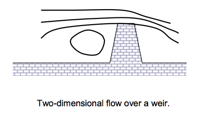
Flow is two-dimensional if it can be assumed that the flow parameters vary in the direction of flow and in one direction at right angles to this direction. Streamlines in two-dimensional flow are curved lines on a plane and are the same on all parallel planes. An example is flow over a weir for which typical streamlines can be seen in the figure below. Over the majority of the length of the weir the flow is the same - only at the two ends does it change slightly. Here correction factors may be applied.
In this course we will only be considering steady, incompressible one and two - dimensional flow.
4.3.3 Three-dimensional flow
In analysing fluid flow it is useful to visualise the flow pattern. This can be done by drawing lines joining points of equal velocity - velocity contours. These lines are known as streamlines. Here is a simple example of the streamlines around a cross- section of an aircraft wing shaped body:
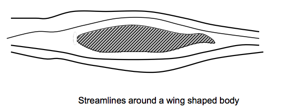
When fluid is flowing past a solid boundary, e.g. the surface of an aerofoil or the wall of a pipe, fluid obviously does not flow into or out of the surface. So very close to a boundary wall the flow direction must be parallel to the boundary.
At all points the direction of the streamline is the direction of the fluid velocity: this is how they are defined. Close to the wall the velocity is parallel to the wall so the streamline is also parallel to the wall. It is also important to recognise that the position of streamlines can change with time - this is the case in unsteady flow. In steady flow, the position of streamlines does not change.
Some things to know about streamlines
- ● Because the fluid is moving in the same direction as the streamlines, fluid can not cross a streamline.
● Streamlines can not cross each other. If they were to cross this would indicate two different velocities at the same point. This is not physically possible.
● The above point implies that any particles of fluid starting on one streamline will stay on that same streamline throughout the fluid.
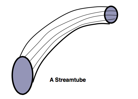
A useful technique in fluid flow analysis is to consider only a part of the total fluid in isolation from the rest. This can be done by imagining a tubular surface formed by streamlines along which the fluid flows. This tubular surface is known as a streamtube.
And in a two-dimensional flow we have a streamtube which is flat (in the plane of the paper):
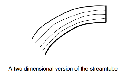
The “walls” of a streamtube are made of streamlines. As we have seen above, fluid cannot flow across a streamline, so fluid cannot cross a streamtube wall. The streamtube can often be viewed as a solid walled pipe. A streamtube is not a pipe - it differs in unsteady flow as the walls will move with time. And it differs because the “wall” is moving with the fluid. -
- 4.4 Mass flow rate
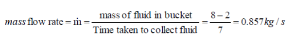
- If we want to measure the rate at which water is flowing along a pipe. A very simple way of doing this is to catch all the water coming out of the pipe in a bucket over a fixed time period. Measuring the weight of the water in the bucket and dividing this by the time taken to collect this water gives a rate of accumulation of mass. This is know as the mass flow rate.
For example an empty bucket weighs 2.0kg. After 7 seconds of collecting water the bucket weighs 8.0kg, then:
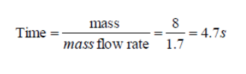
Performing a similar calculation, if we know the mass flow is 1.7kg/s, how long will it take to fill a container with 8kg of fluid?
-
- Volume flow rate - Discharge.
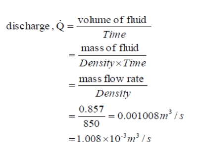
- More commonly we need to know the volume flow rate - this is more commonly known as discharge. (It is also commonly, but inaccurately, simply called flow rate). The symbol normally used for discharge is Q. The discharge is the volume of fluid flowing per unit time. Multiplying this by the density of the fluid gives us the mass flow rate. Consequently, if the density of the fluid in the above example is 850 kg/m3 then:
An important aside about units should be made here:
As has already been stressed, we must always use a consistent set of units when applying values to equations. It would make sense therefore to always quote the values in this consistent set. This set of units will be the SI units. Unfortunately, and this is the case above, these actual practical values are very small or very large (0.001008m3/s is very small). These numbers are difficult to imagine physically. In these cases it is useful to use derived units, and in the case above the useful derived unit is the litre. (1 litre = 1.0×10⁻³ m3). So the solution becomes 1.008 l/s. It is far easier to imagine 1 litre than 1.0×10⁻³ m3. Units must always be checked, and converted if necessary to a consistent set before using in an equation. -
- Discharge and mean velocity.
- If we know the size of a pipe, and we know the discharge, we can deduce the mean velocity
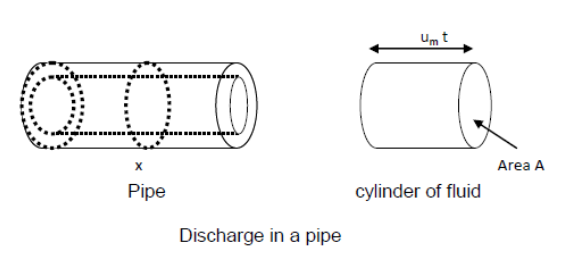
If the area of cross section of the pipe at point X is A, and the mean velocity here is um . During a time t, a cylinder of fluid will pass point X with a volume A×um×t. The volume per unit time (the discharge) will thus be
V = A x um -
- Continuity of flow
Matter cannot be created or destroyed - (it is simply changed in to a different form of matter). This principle is known as the conservation of mass and we use it in the analysis of flowing fluids. The principle is applied to fixed volumes, known as control volumes (or surfaces), like that in the figure below:
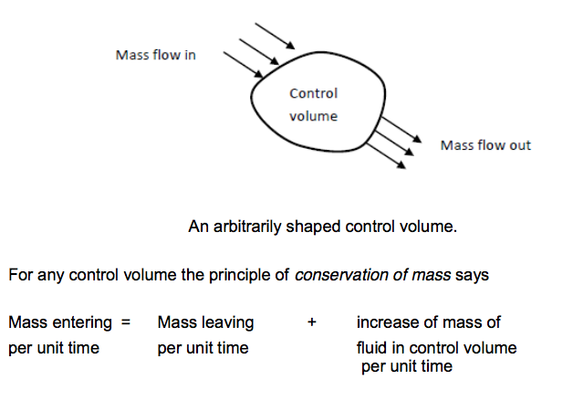
For steady flow there is no increase in the mass within the control volume, so
Mass entering per unit time = Mass leaving per unit time
This can be applied to a streamtube such as that shown below. No fluid flows across the boundary made by the streamlines so mass only enters and leaves through the two ends of this streamtube section.
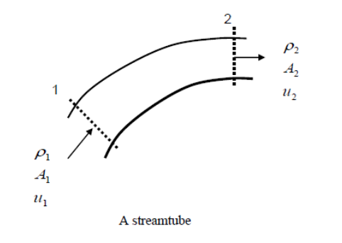
We can then write
mass entering per unit time at 1 = mass leaving per unit time at 2
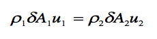
Or for steady flow,
This above equation is known as the continuity of flow equation.
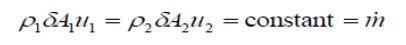
The flow of fluid through a real pipe (or any other vessel) will vary due to the presence of a wall - in this case we can use the mean velocity and write.
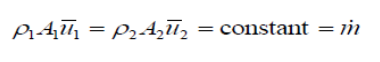
When the fluid can be considered incompressible, i.e. the density does not change, ρ1 = ρ2 = ρ so (note that 𝑢̅ refers to mean velocity)
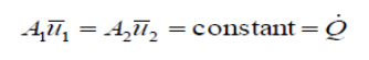
This is the form of the continuity equation most often used. 𝑄̇ is known as volume flow rate (m3/s). This equation is a very powerful tool in fluid mechanics and will be used repeatedly throughout the rest of this course.
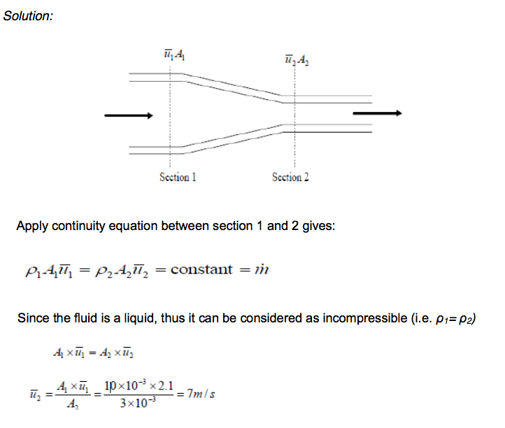
Example:
A liquid is flowing from left to right. Given that the area A1=10×10-3 m2, A2 = 3×10⁻³ m2, and the upstream mean velocity u1 = 2.1 m/s. determine the downstream mean velocity.
-
- 4.8 Velocities in branched pipes and junctions
- The continuity equation is one of the major tools of fluid mechanics, providing a means of calculating velocities at different points in a system. Also it can be applied to determine the relation between the flows into and out of a junction, in the figure shown below for steady conditions,
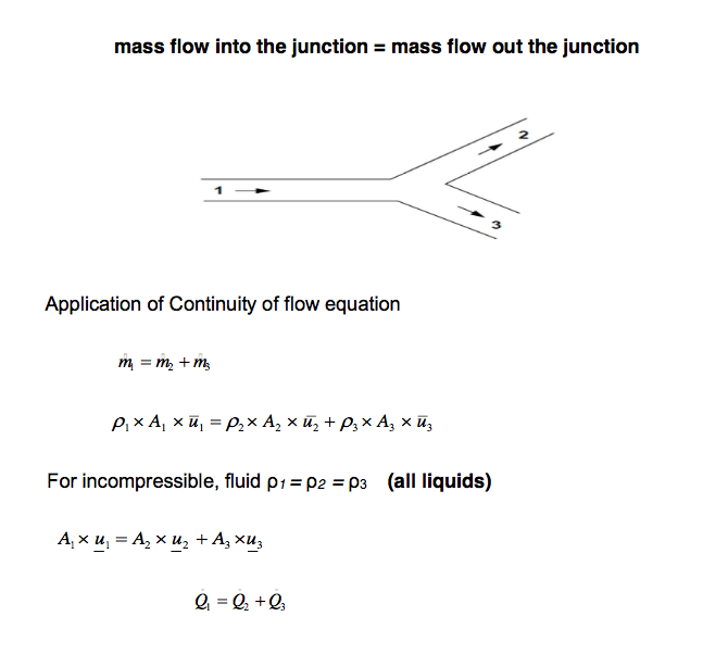
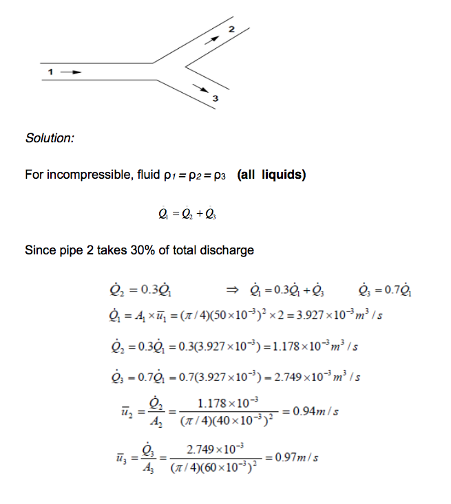
Example:
The branched pipe shown in Figure below carries water. Given that pipe 1 diameter = 50mm, mean velocity 2 m/s, pipe 2 diameter 40mm takes 30% of total discharge and pipe 3 diameter 60mm. Determine the values of discharge and mean velocity in each pipe.
Week 4 Activities 1-4
4 activity with randomized numbers and tasks using MapleTA -
- Summary
- This week, we introduced the concepts necessary to analyse fluids in motion and identified the differences between Steady/unsteady, uniform/non-uniform and compressible/incompressible flow. We demonstrated streamlines and stream tubes. We also introduced the Continuity principle and demonstrated its practical uses in the analysis of flow, eg. fluid flow in branched pipes.
-