01
-
- REVIEW OF BASIC CIRCUIT THEORY
- • Introduction
• SI Units and Common Prefixes
• Electric Current
• Direct Current (DC) and Alternating Current (AC)
• Voltage and Voltage Sources
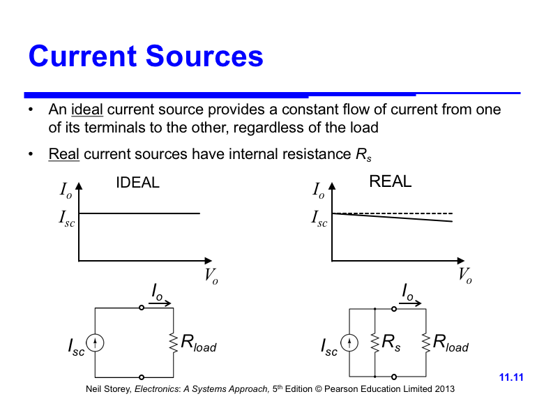
• Current Sources
• Resistors (Ohm’s Law and Power Dissipation)
• Kirchhoff’s Laws
• DC Circuits
• Network Theorems
• AC Circuits (& Complex Numbers)
- Introduction
- • This lecture outlines the basics of Electrical Circuits
• For most students much of this will be familiar this lecture can be seen as a revision session for this material
• If there are any topics that you are unsure of (or that are new to you) you should get to grips with this material BEFORE the next lecture.
- the following lectures will assume a basic understanding of these topics. -
Common Prefixes
Prefix Name Meaning (multiply by) T tera 1012 G giga 109 M mega 106 k kilo 103 m milli 10-3 µ micro 10-6 n nano 10-9 p pico 10-12 SI Units
Quantity Quantity symbol Unit Unit symbol Capacitance C Farad F Charge Q Coulomb C Current I Ampere A Electromotive force E Volt V Frequency f Hertz Hz Inductance (self) L Henry H Period T Second s Potential difference V Volt V Power P Watt W Resistance R Ohm Ω Temperature T Kelvin K Time t Second s
-
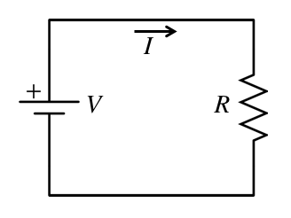
- Electric Current
- • Current is the flow of charge:
• Conventional current assumes the flow of positive charge.
• In practice the charges that flow are usually electrons having negative charge.
• They flow in the opposite direction to that of the conventional current.
• To have a current we need a voltage source and a closed path.
• Units: amperes or “amps” (A)
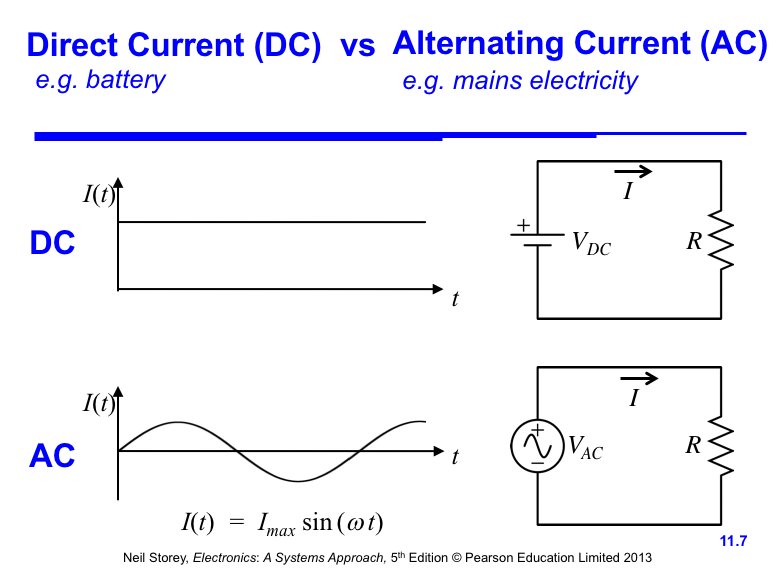
- Direct Current and Alternating Current
- Currents in electrical circuits may be constant or may vary with time
• When currents vary with time they may be unidirectional or alternating
• When the current flowing in a conductor always flows in the same direction this is direct current (DC)
• When the direction of the current periodically changes this is alternating current (AC)
-
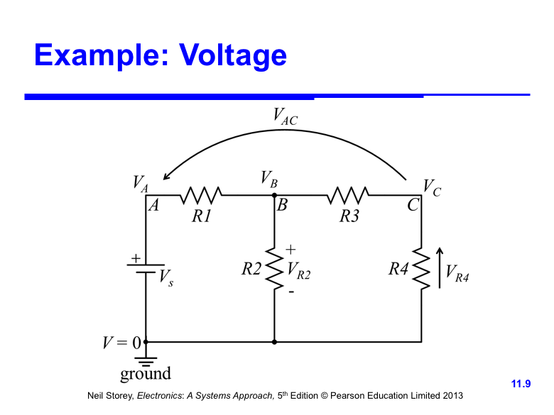
- Voltage
- • Voltage = Potential Difference
• Every point in a circuit is at a particular potential
• Some point (usually the negative terminal of the power supply) is assigned zero potential and called the GROUND
• Hence every point in a circuit has a particular voltage with respect to ground (voltage at a point)
• There is also a voltage between any two points in a circuit (VAB , voltage between A and B)
• There is a voltage across every circuit element (VR1 , VR2 , etc.)
• The voltage between two points or across a circuit element is indicated by polarity signs or by an arrow indicating the direction of potential increase
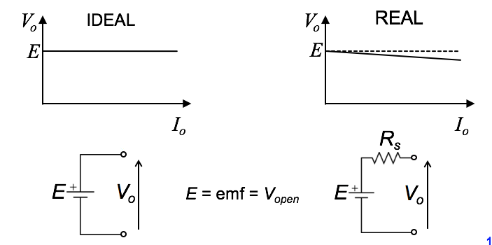
- Voltage Sources
- • An ideal voltage source maintains a constant voltage between its two terminals regardless of the output current
• Real voltage sources (e.g. a battery) have internal resistance Rs
-
- Resistors
- • A resistor is anything that follows OHM’S LAW
• Ohms Law : V ∝ I
- constant of proportionality is the resistance R
- hence
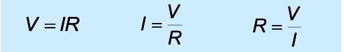
- current through a resistor causes power dissipation
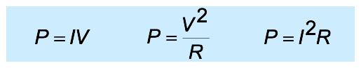
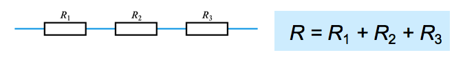
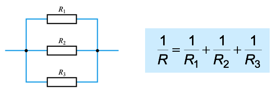
- Resistors in Series and Parallel
- • Series (same current)
• Parallel (same voltage)
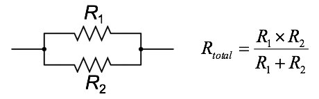
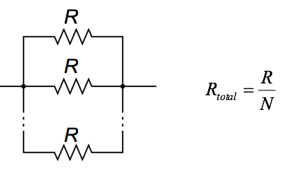
- Resistors in Parallel – special cases
- • Any Two Resistors
N Equal Resistors
-
- Kirchhoff’s Laws
Watch Video (1) 📹
Watch Video (2) 📹
- Node
a point in a circuit where two or more circuit components are joined
Loop
any closed path that passes through no node more than once
Mesh
a loop that contains NO other loop
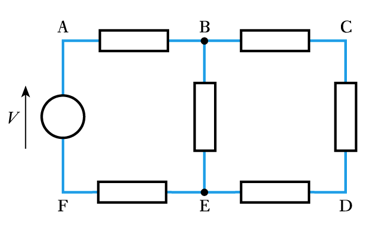
Examples:
A, B, C, D, E and F are nodes the paths ABEFA, BCDEB and ABCDEFA are loops ABEFA and BCDEB are meshes
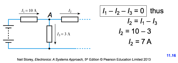
- Kirchhoff’s Current Law
- ● At any instant the algebraic sum of the currents flowing into any junction or node in a circuit is zero
● For any node Σ I = 0
● For example, for node A
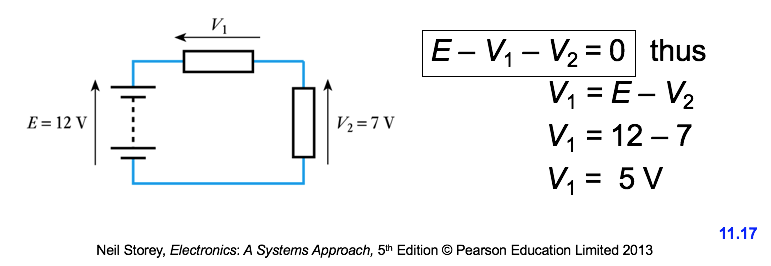
- Kirchhoff’s Voltage Law
- ● At any instant the algebraic sum of the voltages around any loop in a circuit is zero
● For any loop Σ V = 0
● For example, for the single-loop circuit below
-
- DC Circuits
- ● DC circuits involve only resistors, since for DC, inductors behave as short circuits and capacitors as open circuits
● The best way to review DC circuit analysis and Kirchhoff’s laws is by using an example circuit
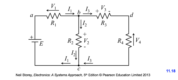
- Find All the Currents and Voltages
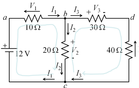
Apply KVL to the RHS loop cabc : 12 - V1 - V2 = 0
Apply KVL to the LHS loop cbdc : V2 - V3 - V4 = 0
Using Ohm’s law, the two equations become
12 - 10 I1 - 20 I2 = 0
20 I2 - 30 I3 - 40 I3 = 0
Apply KCL to node b
I1 - I2 - I3 = 0
We have 3 equations with 3 unknowns
These system of equations must be solved (maths, computer) to find I1 , I2 and I3
Then use Ohm’s law to find the voltages across the resistors (V1 = 10 I1 , V4 = 40 I3 , etc.)
- Voltage Divider
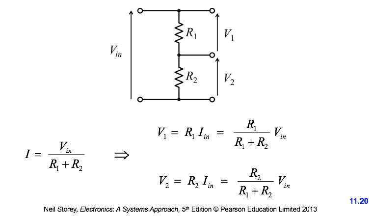
-
- Thévenin’s and Norton’s Theorems
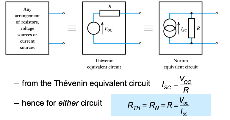
- Thévenin’s Theorem
As far as its appearance from outside is concerned, any two-terminal network of resistors and energy sources can be replaced by a series combination of an ideal voltage source VTH and a resistor RTH , where VTH is the open-circuit voltage of the network and RTH is the resistance that would be measured between the output terminals if the internal energy sources were set to zero.
Note: An (ideal) voltage source is set to zero replacing it with a short circuit, while an ideal current source is set to zero replacing it with an open circuit
- Example – (see Example 3.3 from course text)
Determine Thévenin and Norton equivalent circuits of the following circuit
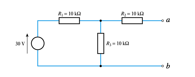
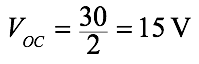
- if nothing is connected across the output no current will flow in R2 so there will be no voltage drop across it. Hence Vo is determined by the voltage source and the potential divider formed by R1 and R3. Hence -
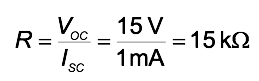
- if the output is shorted to ground, R2 is in parallel with R3 and the current taken from the source is 30V/15 k Ω = 2 mA.
This will divide equally between R2 and R3 so the output current Isc=1mA
the resistance in the equivalent circuit is therefore given by
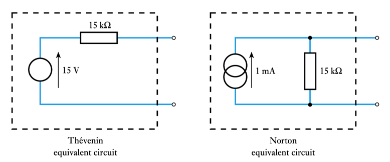
- hence equivalent circuits are:
-
- Superposition Theorem
- Superposition Theorem
In any linear network of resistors, voltage sources and current sources, each voltage and current in the circuit is equal to the algebraic sum of the voltages or currents that would be present if each source were to be considered separately, with all the other sources set equal to zero.
Note: An (ideal) voltage source is set to zero replacing it with a short circuit. An (ideal) current source is set to zero replacing it with an open circuit
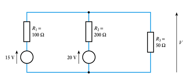
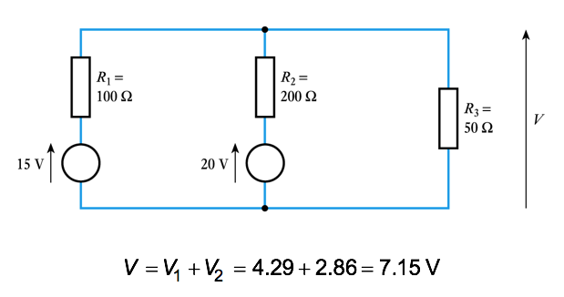
Example -– (see Example 3.5 from course text)
Determine the voltage V of the following circuit
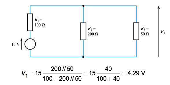
- - first consider the effect of the 15 V source alone, call it V1
- the 20 V voltage source is set to zero replacing it with a short circuit
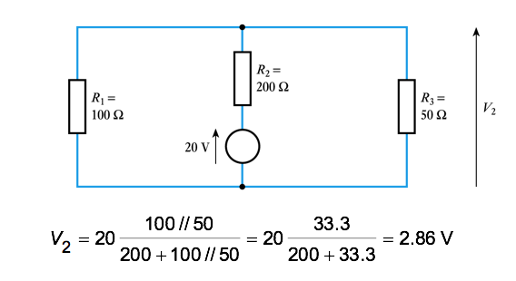
 - now consider the effect of the 20 V source alone , call it V2
- the 15 V voltage source is set to zero replacing it with a short circuit
- the output of the total voltage V is the sum of these two voltages
-
- AC Circuits
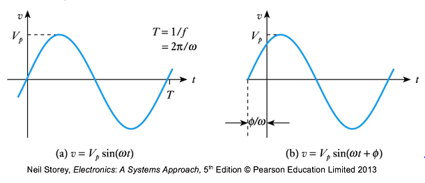
- ● In AC circuits, all voltages and currents are sinusoidal signals
● Sine waves are characterised by three quantities
- Amplitude or peak value (Vp )
- Frequency (linear f or angular ω = 2Πf ). Period T = 1/f
- Phase angle Φ
● We want to find the amplitude AND phase of all voltages and currents (the frequency ω is the same)
● To do this we use COMPLEX NUMBERS -
- Complex Numbers (Appendix D of Storey book)
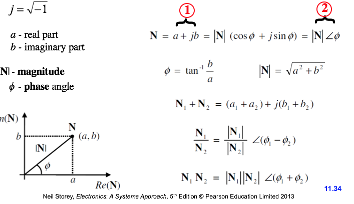
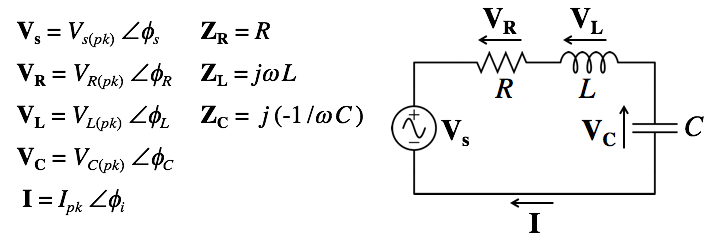
- AC Circuits
● We associate every sine wave with a complex number representation (sometimes called phasor)
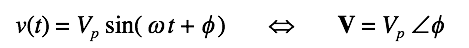
-
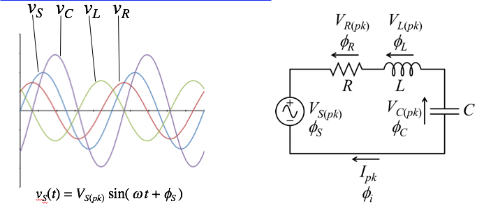
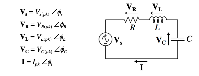
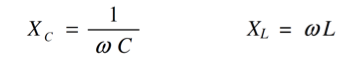
- Impedance and Reactance
- While in DC circuits we use resistance, in AC circuits we use impedance
Z = V / I
It is a complex number defined in the general case of a series RLC combination, as
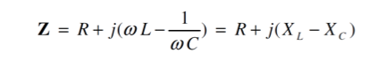
XL & XC are the inductive and capacitive reactances
- AC Circuits
● Once everything is in complex number form (i.e. phasors and impedances) we can apply the same techniques and laws used for DC circuits, except we have to use complex algebra to do the operations
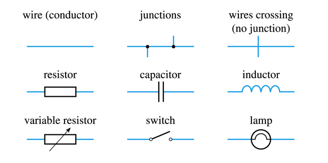
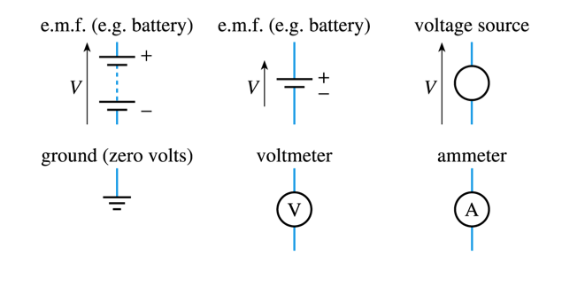
- Circuit Symbols
-
- Key Points
- ● Understanding the next few lectures of this course relies on understanding the various topics covered in this session
● A clear understanding of the concepts of voltage and current is essential
● Ohm’s Law and Kirchhoff’s Laws are used extensively in later lectures
● Experience shows that students have most problems with potential dividers - a topic that is used widely in the next few lectures
● You are advised to make sure you are happy with this material now -
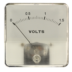
- Measuring Voltages and Currents
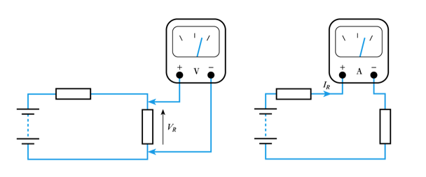
- Measuring voltage and current in a circuit
- when measuring voltage we connect across the component (in parallel)
- when measuring current we connect in series with the component
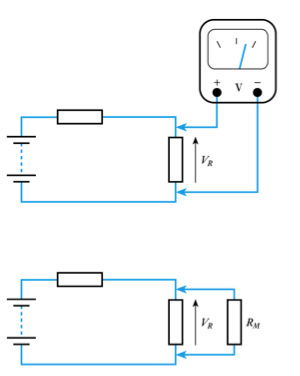
Loading effects - voltage measurement
- our measuring instrument will have an effective resistance (RM)
- when measuring voltage we connect a resistance in parallel with the component concerned which changes the resistance in the circuit and therefore changes the voltage we are trying to measure
- this effect is known as loading
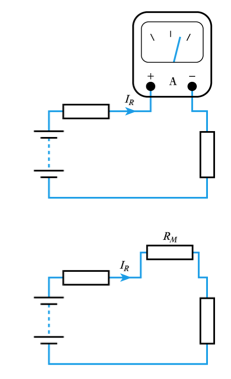
- Loading effects - current measurement
- - our measuring instrument will have an effective resistance (RM)
- when measuring current we connect a resistance in series with the component concerned which again changes the resistance in the circuit and therefore changes the current we are trying to measure
- this is again a loading effect
-
- Oscilloscopes
- An oscilloscope displays voltage waveforms
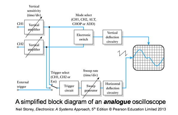
A typical analogue oscilloscope
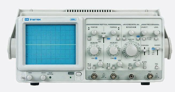
Read Appendix A of Keysight “DSO Lab Guide and Tutorial”
http://literature.cdn.keysight.com/litweb/pdf/54136-97000.pdf
- Further Study
- ● The Further Study section at the end of Chapter 2 looks at the measurement of different forms of alternating waveform.
● Have a look at the problem and then watch the video to see how you did.
Watch The Video 📹
-
- Engineering Systems

● Introduction
● A Systems Approach to Engineering
● Systems
● System Inputs and Outputs
● Physical Quantities and Electrical Signals
● System Block Diagrams
- Introduction
- ● Electronic systems have found their way into almost every aspect of our lives
● In many cases electronic systems are used since they offer a cost effective solution
● In others they offer the only solution
● Few if any systems are entirely electronic
● In practice all real engineering systems are interdisciplinary in nature and involve a wide range of engineering skills and techniques
- A Systems Approach to Engineering
- ● Engineering systems are often very complex
● One approach is to adopt a systematic approach
- complex systems divided into a number of elements
- a top-down approach
- a ‘reductionist’ view
- assumes that a system is no more than the sum of its parts
- however, some system features relate to the interaction of many system elements ◇ e.g. the ‘ride’ or ‘feel’ of a car is not determined by one part
A systemic approach looks at characteristics of the complete system
Modern engineering practice has developed a more ‘holistic’ approach to engineering that combines ‘systematic’ and ‘systemic’ elements - this is termed a systems approach
- has its origins back in the 1960s
- has become widely used only recently
- includes strong emphasis on the application of scientific methods and an interdisciplinary approach
- Systems
- ● A system can be defined as 'Any closed volume for which all the inputs and output are known'
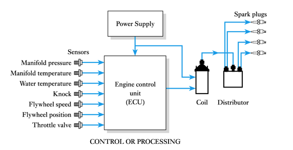
● Examples include:
- an engine management system
- an automotive system
- a transportation system
- an ecosystem
● Inputs and outputs will reflect the nature of the system -
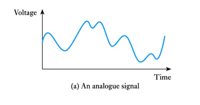
- Physical Quantities & Electrical Signals
- ● The world about us is characterised by a number of physical properties or quantities e.g. temperature, pressure, humidity, etc.
● Physical quantities may be continuous or discrete.
● Continuous quantities change smoothly and can take an infinite number of values
● Discrete quantities change abruptly from one value to another.
- most real-world quantities are continuous
- many man-made quantities are discrete
● It is often convenient to represent physical quantities by electrical signals. These can also be continuous or discrete
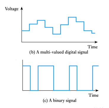
● Continuous signals are often described as analogue
- ● Discrete signals are often described as digital signals
● Many digital signals take only two values and are referred to as binary signals
-
- System Inputs and Outputs
- ● Systems may often be described simply by their inputs, their output and the relationship between them
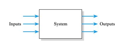
● Nature of inputs/outputs will depend on where we draw our system boundaries. For example:
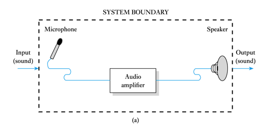
- ● By changing the system boundary we change the nature of the inputs and outputs
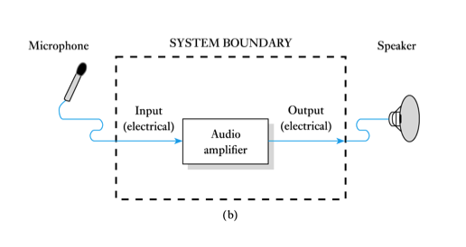
● Components that interact with the outside world are termed sensors and actuators
- in the previous example the microphone represents a sensor
- in the previous example the loudspeaker represents an actuator
● We will look at sensors and actuators in more detail in later lectures -
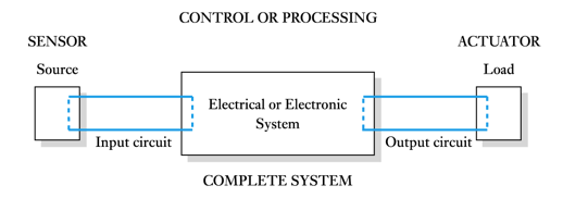
- System Block Diagrams
- ● It is often convenient to represent complex arrangements by a simplified block diagram
● In an electrical system a flow of energy requires a circuit - a system with a single input and a single output is shown below
- this shows the input circuit and the output circuit
- the sensor represents the source
- the actuator represents the load
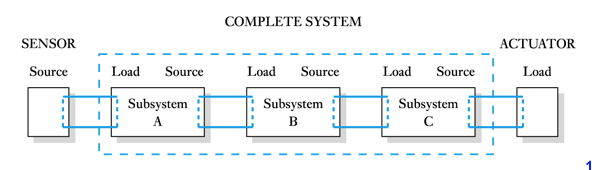
- ● We often divide complex circuits into subsystems or modules – as shown below
- the output of each module represents a source for the following section
- the input of each module represents a load to the previous section
- Key Points
- ● Engineering is inherently interdisciplinary
● Engineers often adopt a ‘systems approach’
● Systems may be defined by their inputs, their outputs and the relationship between them
● Systems interact with the world using sensors and actuators
● Physical quantities can be either continuous or discrete
● Physical quantities are often represented by signals
● Complex systems are often represented by block diagrams -
-
-
-