11
-
Introduction
- By the end of this Section you will be in a position to demonstrate that you can
- explain the factors used in determining the economics of the supply system.
- explain how supply is matched to load demand
- interpret a supply authority's industrial tariff and compute monthly bills.
- In order to do some worked examples in Section 4.3 you will need to have a current tariff sheet. You can get this from a shop or office of your local supply authority.
The Economics Of The Supply System
- In this section seven important factors associated with supply system economics are identified and defined.
- The annual cost of operating a national supply system is based on exactly the same factors as any other business which provides an end-product or service to a consumer. These basic costs can usually be divided into two parts, fixed costs and variable costs.
- a fixed cost is largely independent of energy output
- a variable cost varies directly in proportion to output.
Fixed Costs
- We'll take the example of a single large power station by way of introduction to the fixed costs which apply to the industry as a whole.
- Fixed costs are incurred independently of whether the annual energy output of the station is high or low. That is they are independent of actual output. They include
- salaries - of maintenance staff and engineers
- maintenance materials for buildings and plant as well as running spares
- interest paid annual.ly on money borrowed for construction of a power station or transmission line
- depreciation allowance or sinking fund which is money put aside to replace old plant as it reaches the end of its useful life.
- All these have to be paid for whether or not the power station is contributing much to the National Grid but if they were neglected it would obviously.affect the station's ability to produce a high output - its possible output.
- Another group of fixed costs is largely independent of both actual and possible output. These are:
- Administration
.- Publicity & Marketing
- Design & Development
- So, none of the costs in the bulleted lists is directly proportional to the number of units generated per annum.
- Fixed costs are sometimes referred to as capital costs or standing charges.
Variable Costs
- A variable (or running) cost is directly related to the annual energy output and in the case of power stations is mainly the cost of fuel and water.
- In practice it can be difficult to separate fixed and variable costs precisely. For example, the cost of maintenance does partly depend on the number of units generated per annum.
-
Activity 1
- If the actual maximum demand at any one time is typically 60 GW, what diversity factor should you apply?
- Reveal Solution
Comment on Activity 1
- Diversityfactor = \frac{sum~of~all~possible~demands}{actual~demand}
- Diversityfactor = \frac {300}{60}
- Diversityfactor = 5
Activity 2
- Imagine you live in a rural area and are one of six houses supplied from an 11 kV radial feeder. You can work out the diversity factor which the supply authority has applied to the collective installation.
- Look around your house and note the rating of all the electrical appliances then imagine a high load situation such as a dismal winter Sunday morning when, perhaps, the electric cooker is heavily used, immersion heater on, numerous lights, entertainment equipment, extra heating, washing machine and tumble dryer, kettle, hair dryer, vacuum cleaner and so on. (This is your domestic maximum demand.)
- Add up these loadings and multiply by 6 for all the houses.
- If the power factor is to be near enough unity, then the total kW for the collective installation will be the total kVA.
- H the houses are fed from an 11 kV/240 V, 45 kVA single phase transformer, find the diversity factor which has been applied.
- Reveal Solution
Comment on Activity 2
- Diversityfactor = \frac{sum~of~all~possible~demands}{actual~demand}
- Since the supply authority has seen fit to install a 45 kVA transformer diversity
- factor applied by the supply authority
- = \frac{sum~of~your~possible~demand~x~6}{45~kVA}
- = whatever~you~got!~(should~be~around~5-7)
- Two other factors called the Load Factor and the Power Factor must be considered when the amount of generating and other plant to be installed is being decided.
Diversity Factor
- ln fact, this state of affairs is highly unlikely. It is always the case that when a piece of equipment is manually or automatically switched on, another piece of equipment is switched off somewhere else. So, in practice, a diversity factor can be applied.
- Diversityfactor = \frac{sum~of~all~possible~demands}{actual~demand}
Activity 3:
- Referring to the variation in Load Demand diagram and looking at A, the area under the curve;
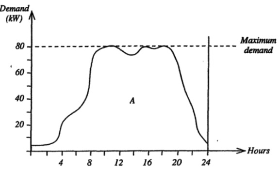
- Diagram 1: Variation in Load Demand
- (a) What does it represent
- (b) Estimate the load factor for this customer
- Reveal Solution
Comment on Activity 3:
- The area under the curve A is equal to the units (i.e. energy) used in the 24 hours. As you can see. this represents about 50% of the maximum possible energy use.
- In other words, the load factor is about 50%
Activity 4:
- Using the domestic maximum demand found in activity 2, work out your load factor (LF) by looking at your last electricity bill to determine the number of units used in the last quarter and dividing by the maximum demand (MD) x number of hours in the quarter.
- i.e. ~ LF = \frac{Number~of~units~used}{MD \times 24 \times days~in~quarter}
- Reveal Solution
Comment on Activity 4:
- You will find that domestic load factors are very poor, perhaps of the order of 0.05.
- If yours is of, say 0.25, you are a 'good' customer. Try asking for a substantial refund!
- The loading in Diagram 2 below uses the same number of units in the 24 hours but the loading is steady. This results in an ideal load factor of 100%. You'll notice that steady loading lowers the maximum demand to 50% of that in Diagram 1
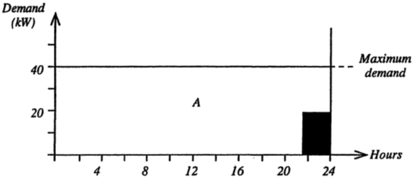
- Diagram 2: Load Factor of 100%
- 100% load factor is difficult to achieve in practice but by comparing Diagram 1 and 2 you can see how any improvement usually releases supply authorities' equipment through reducing demand thereby making a supply available to other consumers without the addition of more plant.
-
Load Factor
- Load factor is defined as the energy consumed in a given period compared with the energy which would have been consumed if the maximum demand had been sustained during that period.
- So that for any given period
- Load Factor ...
- \frac{Energy~consumed}{Energy~which~would~have~been~consumed~had~maximum~demand~been~sustained}
- The following diagram illustrates the importance of load factor.
Variation in Load Demand
- Diagram 1: Variation in Load Demand
- The above diagram shows a consumer’s loading with high peaks and also times of light load during one day (the 24 hour cycle).
Power Factor
- A low or poor Power Factor will require a high current for a given power. It is assumed here that you are familiar with the term Power Factor and aware of the implications of a poor power factor on current demands. If you have any difficulty with this consult your tutor.
- Supply authorities encourage consumers to improve both load factor and power factor. This enables plant rating to be kept within reason and also makes spare capacity available for other consumers and is achieved through well-constructed tariffs.
- 🔗 https://en.wikipedia.org/wiki/Power_factor
Load and Demand
- In order to determine realistically the size of plant required for generation and transmission it is necessary to take into account a number of important factors. All these factors involve - either directly or indirectly - the problem of maximum demand.
- Maximum demand is defined as the actual maximum load on a system during a given period of time (day/month/year). However, consideration must also be given to what might be the maximum demand if all consumers switched on their loads at the same time.
- The domestic evening peak begins when industry and commerce are reaching the end of their working day and some overlap occurs resulting in an overall daily peak indemand between 1800 - 2000 hours.
- As we go about our daily lives our personal demand for energy (directly and indirectly) remains but changes location. For example, as we leave our place of work and switch off lights or equipment or machinery we may take the train home so using electrical energy in another form. At home we light and heat rooms, cook meals, switch on equipment for entertainment, constantly using electrical energy throughout our waking hours.
- The domestic evening peak occurs when industry and commerce are reaching the end of the working day and there is some overlap with increased early evening domestic demand.
- The total possible load for all UK consumers would be in the order of 3000 W. But this would only occur if every consumer made their maximum demand simultaneously.
-
Matching Load Demand and Supply
- This section provides an insight into how the demand for power varies depending on the time of day or season and the facilities available to the Control Engineer attempting to match the output from the generators to the load demand.
- All conventional power stations are listed in order of merit. This is a system of comparing the cost per unit generated between stations so that the low cost plant is used in preference. By taking a number of factors into consideration. such as weather predictions and television 'pick-up', the engineer is able to use the high capital cost/low running cost stations (such as nuclear) as base load plant.
- Electricity, unlike other forms of energy, cannot be easily stored and the supplier has little control over the load at any time. So the control engineers try to keep the output from the generators equal to the connected load at the specified voltage and frequency. A measure of how well they do this is how close the national frequency is to 50 Hz throughout any 24 hours.
- The demand for electricity on a system varies considerably during any 24 hour period and the demand during the winter months is much greater than that in the summer months.
Load Curve
- A load curve is a graphica1 representation of the amount of power supplied by the system against time and the diagram below is a typical example.
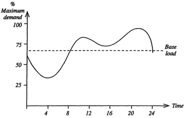
- Diagram 3: Load Curve
- You can see that the daily load consists of a 'base' component plus peaks and troughs depending on the time of day.
Spinning Reserve and Static Reserve
- Sudden peaks are met using spinning reserve and static reserve which can amount to 3000 MW during the day and 1250 MW at night.
Spinning Reserve
- Spinning reserve involves machine sets being run up and synchronised to the system but supplying little or no power.
- Steam boilers are held at full working pressure with sufficient steam passing through the turbines to maintain working temperatures. This enables the set to be fully loaded in a matter of minutes instead of hours as would be the case from cold.
Static Reserve
- Static reserve is provided in two ways.
- i) Some steam sets are kept turning over slowly (a few rpm) by what is known as baring gear, with again sufficient steam passing through to keep the turbine at a reasonable temperature.
- The boiler is kept at somewhat less than full pressure but with enough steam in reserve to enable the set to be run-up and load taken in about an hour. This system is known as Hot Standby.
- ii) Water turbines (hydro power) and large gas turbines are able to run-up from standstill and be fully loaded in a very short time (typically 5 minutes).
- Such sets are invaluable for meeting sudden, unpredicted peak demands and in keeping the system frequency stable. The drawback with hydro generation is the large civil works and water catchment required (typical single set 10 - 20 MW). The disadvantage of gas turbine driven sets on the other hand is the cost of fuel and maintenance together with their short life (typical single set 20 - 30 MW).
- A recent addition to the generation system in the last 20-25 years has been the development of hydraulic pumped storage. This involves a much larger than usual hydro station (typically 400 MW) being supplied from a relatively minute head pond (reservoir).
- At times of peak demand the station generates in the normal manner supplying power to the grid. The tail water runs into a lower pond and not to 'waste' or into a further downstream station on the same scheme as is usually the case with a conventional hydro station.
- At times of low demand the electrical machines are synchronised to the grid but run in reverse so that they drive the water turbines as large pumps. In this way they pump water from the tail pond up into the head pond.
Activity 5:
- Although more costly and complex than a conventional hydro station, hydraulic pumped storage has advantages.
- Can you list 2 or 3 ?
- Reveal Solution
Comment on Activity 5:
- Pumped Storage is able to utilise the spare capacity of large steam stations at what would otherwise be times of light load. This increases the overall efficiency of the system.
- Large amounts of power can be very quickly fed into the grid at times of peak demand.
- If, say, a 400 MW pump storage station is operating in the pumped mode and is instructed to generate, this is effectively 800 MW of capacity available within minutes.
- Sudden large demands on the system will cause the speed of all generating sets to fall. This is sensed by the speed governors. More steam or water is then supplied to the turbines in order to meet the extra load.
- At any one time much rotating machinery is connected to the grid so that a sudden fall in frequency results in a drop in the synchronous speed of all motors and generators. This mass of machinery acts like a huge flywheel and, in addition to spinning and static reserve, presents a useful buffer action so preventing large frequency swings.
- In very difficult conditions, such as loss of a large generating set or severe storm damage, the frequency may fall to an unacceptable level so that automatic or manual load shedding is carried out. This has to be carefully done so as not to jeopardise national security or vital services.
-
Construction and Application of Industrial tariffs
- We now need to examine the way in which large consumers are charged for their electricity supply and how the structure of the tariffs encourages consumers to reduce their maximum demands and improve power factors.
- The maximum demand made on a large supply system determines the size and cost of the installation. You will remember that Load Factor is defined as the energy consumed in a given period compared with the energy which would have been consumed if the maximum demand had been sustained.
- So, for a fixed total annual energy consumption, a low load factor results in a high maximum demand. In tum a high maximum demand results in a high financial cost per electrical unit consumed in terms of supply plant and equipment. Since annual energy consumption is (hopefully) proportional to goods produced and services provided, a high maximum demand means an unnecessarily high cost in a competitive market.
- Well-constructed tariffs are designed to provide the necessary financial incentives to influence consumers.
- They are encouraged to consume a higher proportion of energy at reduced cost. It is quite possible to double the energy consumption (and so double output more or less) and only put 15% to 20% on the electricity bill.
- Financial incentives can reduce overall maximum demands, and consequently the heavy costs associated with just getting a supply to a large consumer.
- Customers who use more energy during the night get cheaper electricity because this keeps the large steam generators operating at or near their most efficient.
- There are incentives to keep demands down during the winter months when an overall upsurge takes place.
- Tariffs are also designed to improve power factors towards unity, so that power stations are only producing and transmission lines are only carrying active power.
Two-Part Tariffs
The tariffs are constructed so that consumers pay charges to meet the various costs of providing a heavy supply (irrespective of how much energy is used). Such charges are termed fixed charges although in practice they can vary considerably month by month. You'll see how this operates when you do the worked examples overleaf. ·- Customers also pay a running charge which depends on the number of units of energy used.
- These two charges together form what is known as a Two-Part Tariff.
Chargeable Maximum Demand Monitoring
Chargeable Maximum Demand is the monitored maximum demand divided by the average power factor for the month and is referred to as the maximum kVA demand.- This is often a preferable system since it takes into account - and charges for - a low power factor. The average power factor is determined by measuring the kW hrs and kVAr hrs over the month.
- i.e.~ average~ \Theta = tan^{-1}kVarhr
- kWhr
- and~average~power~factor = cos~\Theta
- The Running Charge levied (cost per kWhr consumed) is usually dependent on the time of day. There is one charge between 0730 and 2330 and another much reduced charge between 2330 and 0730. Itis also dependent on the time of year, with cheaper summer tariffs.
- Most industrial tariffs are billed on a monthly basis.
Demand Monitoring
- It is important to note the following points.
- For the units reading a running total is maintained. In contrast, once the demand reading has been reset to zero by the meter reader, the recording has been lost for all time.
- As a result, most companies insist that their representative is present when readings are taken.
- Some supply authorities make separate charges for maximum demand and poor power factor, while others combine the two into one charge. When done in this way it will result in an average kVA demand.
- You will recall that
- kVA = \underline{kW}
- p.f.
- To ensure a fair spread of capital cost it is necessary to measure or monitor a heavy consumer's maximum demand. However, many industrial loads demand large amounts of power for short periods - accelerating a motor and its load for instance - so that monitoring instantaneous demand is considered unfair.
- In any event, the national system can cope with short duration heavy demands due to the inertia of all the rotating machinery connected to the grid.
- A more satisfactory solution is to average out the demand over a relatively short time period and refer to this as monitored demand as opposed to instantaneous demand. The time period used by most supply authorities is 30 minutes.
- MonUored Maximum Demand is defined as twice the number of kWhr supplied during any thirty consecutive minutes in any accounting period. Consider the following example.
- A consumer uses 600 kWh between 0900 and 0930.
- Since energy (kWhrs) ... No. of kW x No.of hours monitored then 600 ... No. of kW x t hrs
- So that the average demand between 0900 and 0930 is given by
- No.~of~kW == 600 + f
- = 12pQkW
- In practice between 0900 and 0930 the instantaneous demand may well have exceeded 1200 kW and at other times been much less.
- This maximum demand is divided into blocks of kWhrs and a decreasing scale of charges is applied to successive blocks.
- To monitor the power flowing into a consumer's installation, a special meter is installed at the intake. As energy is used, a pointer moves round a scale driven at twice the speed at which energy (kWh) is used.
- In order to record the average maximum demand, the meter carries a second pointer which is 'pushed' upscale by the first (driven) pointer. The second pointer simply sits at the highest position to which it is pushed.
- At the end of the 30 minute period the first pointer is automatically set to zero. During the next 30 minute period it may or may not reach and cant forward the second pointer, depending on the demand. At the end of the month a meter reader takes the maximum demand reading and resets the second pointer to zero.
Monitored Maximum Demand
- Monitored Maximum Demand is defined as twice the number of kWhr supplied during any thirty consecutive minutes in any accounting period.
- Consider the following example.
- A consumer uses 600 kWh between 0900 and 0930.
- Since energy (kWhrs) = No. of kW x No.of hours monitored
- then 600 = No. of kW x 0.5 hrs
- So that the average demand between 0900 and 0930 is given by
- No. of kW = 600 ÷ 0.5
- = 1200 kW
- In practice between 0900 and 0930 the instantaneous demand may well have exceeded 1200 kW and at other times been much less.
- This maximum demand is divided into blocks of kWhrs and a decreasing scale of charges is applied to successive blocks.
- To monitor the power flowing into a consumer's installation, a special meter is installed at the intake. As energy is used, a pointer moves round a scale driven at twice the speed at which energy (kWh) is used.
- In order to record the average maximum demand, the meter carries a second pointer which is 'pushed' upscale by the first (driven) pointer. The second pointer simply sits at the highest position to which it is pushed.
- At the end of the 30 minute period the first pointer is automatically set to zero. During the next 30 minute period it may or may not reach and carry forward the second pointer, depending on the demand. At the end of the month a meter reader takes the maximum demand reading and resets the second pointer to zero.
- It is important to note the following points.
- For the units reading a running total is maintained. In contrast, once the demand reading has been reset to zero by the meter reader, the recording has been lost for all time. As a result. most companies insist that their representative is present when readings are taken.
- Some supply authorities make separate charges for maximum demand and poor power factor, while others combine the two into one charge. When done in this way it will result in an average kVA demand.
- You will recall that kVA = kW
- Chargeable Maximum Demand is the monitored maximum demand divided by the average power factor for the month and is referred to as the maximum kVA demand. This is often a preferable system since it takes into account - and charges for - a low power factor. The average power factor is determined by measuring the kW hrs and kVAr hrs over the month.
- i.e.~~average~t/J \cdots tan \cdot \frac{kVar~hr}{kW~hr}
- and~average~power~factor == cos~t/J
- The Running Charge levied (cost per kWhr consumed) is usually dependent on the time of day. There is one charge between 0730 and 2330 and another much reduced charge between 2330 and 0730. Itis also dependent on the time of year, with cheaper summer tariffs.
- Most industrial tariffs are billed on a monthly basis.
-
Demand Monitoring
- Demand must be monitored in order to ensure that the two-part tariff is as fair as possible and to encourage large consumers to improve their load factor (i.e. reduce maximum demand). The examples below illustrates the importance of monitoring.
- Two factories are fed from the high voltage grid via transformers.
- The first one belongs to MacIntosh's Highland Clearances, a scrap metal process works. It operates on full load day and night (including weekends) constantly drawing 1000 kW.
- Therefore, at the end of a month. MacIntosh's has consumed
- 1000 kW \times 730 hours = 730 000 kWh = 0.73 \times 106 kWh~of~energy
- The second factory belongs to Ferguson's Jumpers, a firm specialising in knitwear for tall people. It consumes approximately the same amount of energy over the month (say 7 x 10⁵ kWh) but its load is constantly changing.
- Demand fluctuates between 50 kW and 3000 kW, occasionally reaching peaks of 6000 kW. Due to this, the capacity of the lines, cables and transformers must be greater than those supplying MacIntosh's Highland Clearances. The supply authority must therefore invest more capital to serve Ferguson's Jumpers.
- Consequently it is reasonable that Ferguson's Jumpers should pay more for its energy.
- To ensure a fair spread of capital cost it is necessary to measure or monitor a heavy consumer's maximum demand. However, many industrial loads demand large amounts of power for short periods - accelerating a motor and its load for instance - so that monitoring instantaneous demand is considered unfair.
- In any event, the national system can cope with short duration heavy demands due to the inertia of all the rotating machinery connected to the grid.
- A more satisfactory solution is to average out the demand over a relatively short time period and refer to this as monitored demand as opposed to instantaneous demand. The time period used by most supply authorities is 30 minutes.
- Monitored Maximum Demand is defined as twice the number of kWhr supplied during any thirty consecutive minutes in any accounting period. Consider the following example.
- A consumer uses 600 kWh between 0900 and 0930.
- Since energy (kWhrs) = No. of kW x No.of hours monitored
- then 600 = No. of kW x 0.5 hrs
- So that the average demand between 0900 and 0930 is given by
- No. of kW == 600 + 0.5
- = 1200 kW
- In practice between 0900 and 0930 the instantaneous demand may well have exceeded 1200 kW and at other times been much less.
- This maximum demand is divided into blocks of kWhrs and a decreasing scale of charges is applied to successive blocks.
- To monitor the power flowing into a consumer's installation, a special meter is installed at the intake. As energy is used, a pointer moves round a scale driven at twice the speed at which energy (kWh) is used.
- In order to record the average maximum demand, the meter carries a second pointer which is 'pushed' upscale by the first (driven) pointer. The second pointer simply sits at the highest position to which it is pushed.
- At the end of the 30 minute period the first pointer is automatically set to zero. During the next 30 minute period it may or may not reach and carry forward the second pointer, depending on the demand. At the end of the month a meter reader takes the maximum demand reading and resets the second pointer to zero.
- It is important to note the following points.
- For the units reading a running total is maintained. In contrast, once the demand reading has been reset to zero by the meter reader, the recording has been lost for all time.
- As a result, most companies insist that their representative is present when readings are taken.
- Some supply authorities make separate charges for maximum demand and poor power factor, while others combine the two into one charge. When done in this way it will result in an average kVA demand.
- You will recall that
- kVA = \underline{kW}
- p.f.
-
Application of Tariffs: Some Examples
- The following examples are based on the tariff system used by Scottish Hydro Electric pie and are worked using 2016 – 2017charges.
- A copy of the 2016 tariff sheet is enclosed for reference (page 19). You should also have obtained a copy of the current tariffs from your local supply authority shop or office.
- Look at the heading Maximum demand tariff on the 2016 Hydro Electric sheet.
- You will notice four sub-headings (block letters) with charges opposite them depending whether the supply is taken at high or low voltage.
Maximum Demand Tariff Sheet
Maximum Demand Tariff Sheet
- The company may require the customer to enter into a special agreement for a supply of electricity under this tariff.
The Maximum Authorised Capacity
under this tariff is 20kVAFor High Voltage Supply (Code 54) For Low Voltage Supply (Code 55) Availability Charge Per month for each of the first 20 kVA of charge capacity £2.55 £2.55 Per month for each kVA of chargeable capacity in excess of 20 kVA £0.75 £1.04 Demand Charge Per month for each of the first 750 kilowatts of maximum demand made in the month £1.36 £1.43 Per month for each of the next 3250 kilowatts of maximum demand made in the month £0.60 £1.36 Per month for each kilowatt of maximum demand in excess of 4000 kilowatts made in the month plus per kilowatt of maximum demand made between 0730 and 2330 hours in each of the months mainly in £0.15 £1.36 November and March £3.82 £3.92 December, January and February £7.33 £7.46 The average power factor shall be measured at all times.
Between 2330 and 0730 hours one kilowatt of maximum demand shall be deemed to be half of one kilowatt.Unit Charge For each unit supplied between 0730 and 2330 hours in the months of November to March inclusive 4.77p 5.11p For each unit supplied between 0730 and 2330 hours in the months of April to October inclusive 4.08p 4.27p For each unit supplied between 2330 and 0730 hours 2.50p 2.55p Reactive Kilovoltampere Hours Charge For each kVArh supplied at any time in excess of half the number of units supplied 0.38p 0.59p Catering Charge 0.0667 per kWh Maximum Demand Tariff Sheet
Change of Tariff
- With the consent of the company a customer may change from one tariff to another where alternative Tariffs are available for the particular type of supply, provided that notice in writing is given by the customer to the Company not less than one month before the meter reading from which the alternative Tariff is required to apply, but the date of application of the alternative Tariff will depend on the availability of suitable metering equipment. A customer shall not be entitled to change from one Tariff to another more often than once a year. Full details of these Tariffs are available from our offices and shops.
Value Added Tax
- All charges are inclusive of Value Added Tax which will be charged at the appropriate rate presently at 20%.
Definitions
- Expressions used in this leaflet have the following meanings:
- All times quoted are Greenwich Mean Time.
- The unit of electricity is the kilowatt hour.
- “Authorised Capacity” – means the capacity of supply expressed in kilovoltamperes (kVA) requested by the customer and authorised by the company.
- “Basic Charge” – means for the purpose of the General Tariffs, a sum, payable whether or not electricity is used, in respect of fixed costs associated with the supply of electricity including meter reading and billing costs.
- “Chargeable Capacity” – means the Authorised Capacity of the supply expressed in kilovoltamperes or such higher capacity as may be determined from the recorded maximum demand in kilowatts in the month of the account or in any of the preceding eleven months, whichever is the greater, and the average power factor in the same month.
- “High Voltage Supply” – means a supply metered at more than 1000 volts.
- “Low Voltage Supply” – means a supply metered at 1000 volts or less
- “Maximum Demand” – means twice the largest number of units supplied in any half-hour during a specified charging period. The maximum demand may be addressed by the company in cases where maximum demand indicating equipment is not installed.
- “Month” – means a period of four or five consecutive weeks between one meter reading and the next such reading.
- “Quarter” – means a period of approximately three consecutive months between one meter reading and the next such reading.
- “Reactive kilovoltampere hours” – means the wattles current in the circuit measured over time and is recorded as kVArh.
- “Weekday” – means Mondays to Friday inclusive.
- {The above extract is reproduced by kind permission of Scottish Hydro-Electric plc}
- Availability charge is one of the fixed charges and is based on the capacity of the supply which has been made available to the consumer.
- The following is one way of looking at this. Supposing your area is supplied from a 10 MVA transformer with its associated switchgear, lines and cables. If you have agreed authorised capacity of say 800 kVA then this portion of the network has been reserved for you.
- It is nearly always the case that a consumer asks for, and is granted (on the grounds of future growth), a larger capacity than is really needed. So it may well be that the aforementioned 10 MVA transformer is theoretically fully utilised when in practice its average loading may be as little as 35-40% of its rating.
- In order to feed new consumers without installing new equipment (which usually isn't necessary anyway) the supply authority makes a substantial charge every month for every kVA of authorised capacity. This encourages consumers to be more realistic in their request.
- Since the introduction of the availability charge in the past few years, many consumers have re-submitted requests for unrealistically low capacities and Scottish Hydro Electric have had to be clever in the extreme in dealing with the matter!
-