-
Control Systems: Introduction to Feedback
- What is control?
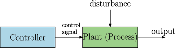
Control systems integrate elements whose function is to maintain a process variable at a desired value or within a desired range of values. A control system generally refers to the methods of adjusting the flow of energy from a source to a load of process so that some desired results may be achieved.- Control system
- Control system input
- Control system output
- Open-loop system
- Closed-loop system
- Controlled variable
- Manipulated variable
- What is control?
-
Open Loop Control System
- An open-loop control system is the one in which the control action is independent of the output. An example of an open-loop control system is a chemical addition pump with a variable speed control as shown in the figure. The feed rate of chemicals that maintain proper chemistry of a system is determined by an operator, who is not part of the control system. If the chemistry of the system changes, the pump cannot respond by adjusting its feed rate (speed) without operator action. The a rate is manipulated by an operator who adjusts the speed of the pump.
📷 Enlarge below Chemical pump system diagram.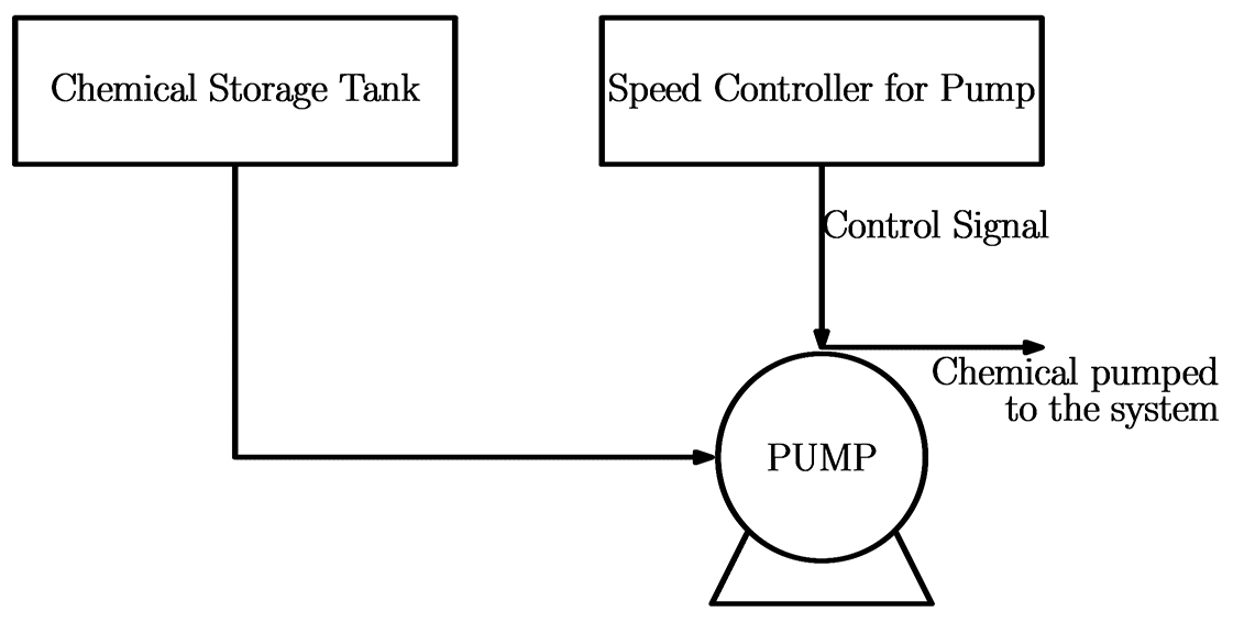 Chemical pump system
Open loop systems
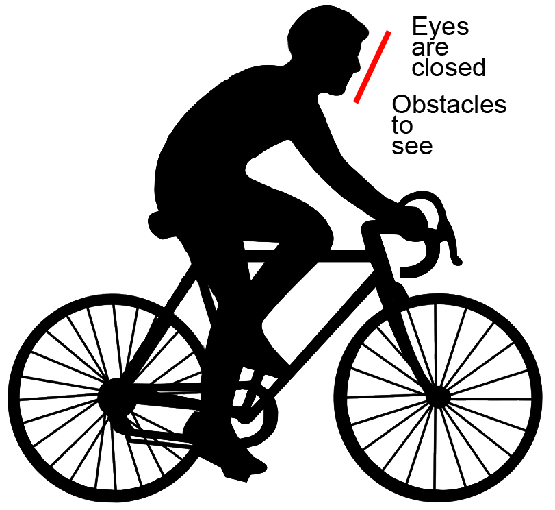
- In an open-loop control system, no feedback from the output is used to control, meaning to adjust the input to, the system. Based on value of the output that is desired, the controller adjusts the input to the plant to achieve this. Control will only work well if plant is highly predictable and there is no internal or external disturbances. Generally used only when good control performance is not required. A very good example of an open loop control system is riding a bike with closed-eyes. Here the eyes are the sensors of the control systems. If the eyes are closed, there will not be any feedback to the person riding the bike.
Open-loop control
Continues on next tab
A typical Control System Example: House heating system
📷 Enlarge below control system diagram.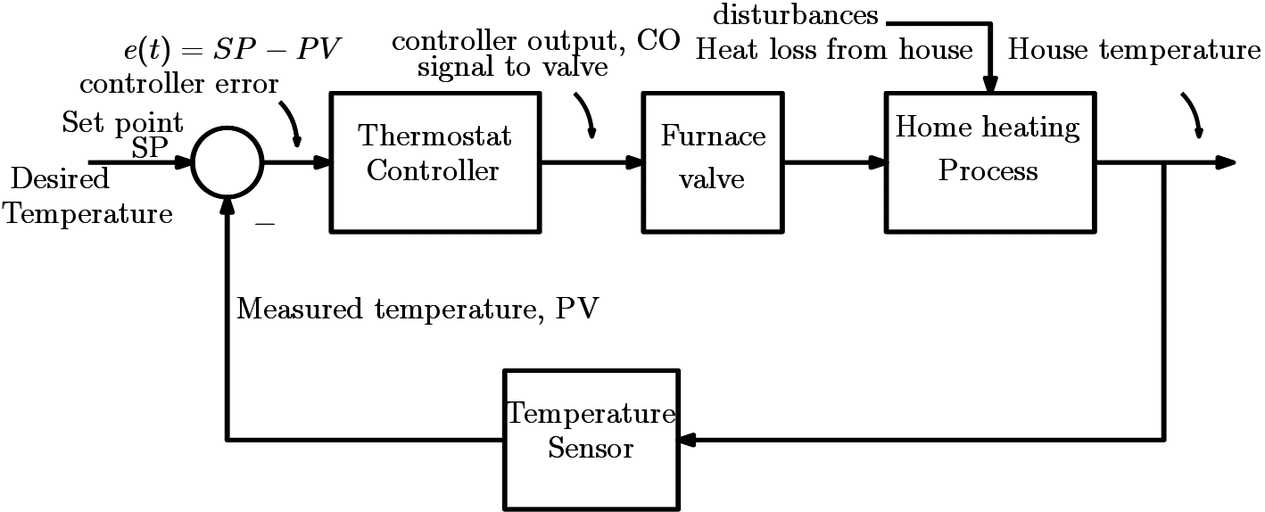
- A control system is a system of integrated elements whose function is to maintain a process variable at a desired value or within a desired range of values. The control system monitors a process variable or variables, then causes some action to occur to maintain the desired system parameter. In the example of the central heating unit, the system monitors the temperature of the house using a thermostat. When the temperature of the house drops to a preset value, the furnace turns on, providing a heat source. The temperature of the house increases until a switch in the thermostat causes the furnace to turn off.
- Control system input
Control system input is the stimulus applied to a control system from an external source to produce a specified response from the control system. In the case of the central heating unit, the control system input is the set point temperature(desired temperature) of the house applied to the control system.
- Control system output
Control system output is the actual response obtained from a control system. In the example above, the temperature dropping to a pre-set value on the thermostat causes the furnace to turn on, providing heat to raise the temperature of the house. Then the control system output is the house temperature.How the heater works
- The room too cold: If the actual room temperature, PV is less than the desired room temperature (SP), a positive error signal ($e(t)$) is generated and the valve opens. This allows the room temperature to rise. i.e. $(SP-PV)=+$
- Room too hot: If the actual room temperature, PV is greater than the desired room temperature (SP), a negative error signal ($e(t)$) is generated and the valve closes. This allows the room temperature to decrease. i.e. $(SP-PV)=-$
- Room at correct temperature: If the actual room temperature, PV is equal to the desired room temperature (SP), a zero error signal ($e(t)$) is generated and the valve does not move. This allows the room temperature to stay at the set point. i.e. $(SP-PV)=0$
- Note Any disturbances such as the heat loss, will cause an error signal which will drive the system to return the error back to zero.
-
When do we use automatic control?
Generally used when good control performance is required.Accurate control can be achieved even in the presence of plant variations, and/or internal or external disturbances.Any such disturbance will affect the output Y and reflected back in the error E. This will cause the plant input U to change so as to correct for the disturbance.Components of a feedback control system
- The aim of the control system
In an automatic control system, the output is continuously monitored by a transducer(sensor) and fed back to the input. The input represents the desired value that the output should reach. The actual output is subtracted from this reference value and the resulting error signal E is used to derive the system towards the required output value. Clearly then the objective isto make the error signal zero which will indicate that the desired output value has been achieved.
- Components: Input Signal(Reference signal) R
This represents the input to the system which produces the desired output effect. For example in an automatic temperature control system this equals to the desired room temperature. For a liquid level control system, this value is equal to the desired liquid height. For a painting robot, this quantity is equal to the (speed and position) trajectory that the spraying mechanism should follow.
- Components: Output Signal(The controlled output) Y
The controlled output is the quantity or condition of the plant which is controlled. This signal represents the controlled variable. The output should follow the input at all times in a effective control system. The output will be a variable such as speed, temperature, position, pressure, Ph level, liquid height, etc. depending on the application.
- Components: Feedback Signal
In modern control systems, the output is continuously monitored using a sensor(transducer). The output of this sensor is called a feedback signal. This signal is fed back to the summing junction for comparison with the desired input. Note that input signals and feedback signals must be of same type. For example if the overall system is a temperature control system, the input should be an electrical signal that is proportional to the temperature. Similarly, the feedback signal must also be an electrical signal that is proportional to the current temperature.
- Components: Controller
The control elements are components needed to generate the appropriate control signal applied to the plant. These elements are also called the "controller." There are many kinds of control systems used in industry. The simplest control system is a proportional control system which generates a control signal directly proportional to the error signal. That is $$U=K\times E$$ Depending on the needs, one can use more advanced control methods.
- Components: Plant(Process)
The plant is the system or process through which a particular quantity or condition is controlled. This is also called the controlled system.
Continues on next tabClosed-loop Control System

- The sensor measures the actual value of the output, Y, compares this with the desired value, R, and computes the error, E. Based on this error E, the controller generates the input, U, to the plant so as to bring Y to the desired value R.
Closed-loop control system: Another example (Heating system)
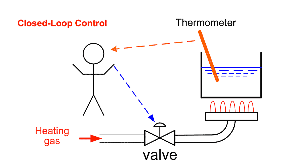
- In this example the operator would like to control the temperature of the water by adjusting the valve which controls the heating gas flow. The sensor that is used to feedback the current temperature is the thermometer. The operator checks the value of the thermometer in regular time intervals and adjust the valve. If the temperature of the the water is less than the desired temperature, the operator turns on the valve and if the temperature is higher than the desired temperature, the operator throttle down the valve.
Not every closed-loop system is automatic control
- Note
In general, not every closed-loop system can be called an automatic control system. In order to call a closed-loop control system as an automatic control system, the controller must not be a human being. For example consider the bicycle riding process (described on tab 11.1). In this system, although there is a feedback via the eyes of the person, the main control mechanism is the person who rides the bike. Therefore this system cannot be called an automatic control system. But if we replace the person with a robot then this system is called and automatic control system.

2 Sets of Reading obtained by 2 different measurement devices of the same quality Instrument 1 20.1mm 20.2mm 20.0mm 20.1mm 20.1mm 20.1mm 20.0mm Instrument 2 19.9mm 20.3mm 20.0mm 20.5mm 20.2mm 19.8mm 20.3mm

- The aim of the control system
-
Block diagrams
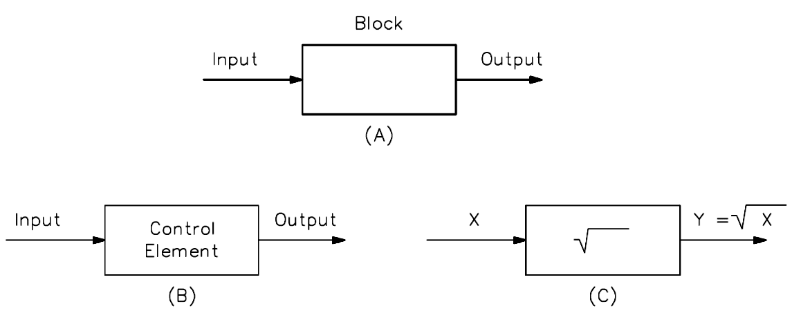
- A block diagram is a pictorial representation of the cause and effect relationship between the input and output of a physical system. A block diagram provides a means to easily identify the functional relationships among the various components of a control system. The simplest form of a block diagram is the block and arrows diagram. It consists of a single block with one input and one output (Figure A). The block normally contains the name of the element (Figure B) or the symbol of a mathematical operation (Figure C) to be performed on the input to obtain the desired output. Arrows identify the direction of information or signal flow.
Takeoff points in block diagrams
- Definition
A takeoff point is used to allow a signal to be used by more than one block or summing point.
- Example 1A:
📷 Temperature control of lubricating oil
- Example 1B:
📷 Temperature control of lubricating oil (cont.)
- Example 1C:
📷 Temperature control of lubricating oil (cont.)
- Example 1D:
📷 Temperature control of lubricating oil (cont.)- Figure shows a typical application of a block diagram to identify the operation of a temperature control system for lubricating oil. (A) shows a schematic diagram of the lube oil cooler and its associated temperature control system. (B) shows the block diagram of the system. Lubricating oil reduces friction between moving mechanical parts and also removes heat from the components. As a result, the oil becomes hot. This heat is removed from the lube oil by a cooler to prevent both breakdown of the oil and damage to the mechanical components it serves.
The lube oil cooler consists of a hollow shell with several tubes running through it. Cooling water flows inside the shell of the cooler and around the outside of the tubes. Lube oil flows inside the tubes. The water and lube oil never make physical contact.
As the water flows through the shell side of the cooler, it picks up heat from the lube oil through the tubes. This cools the lube oil and warms the cooling water as it leaves the cooler.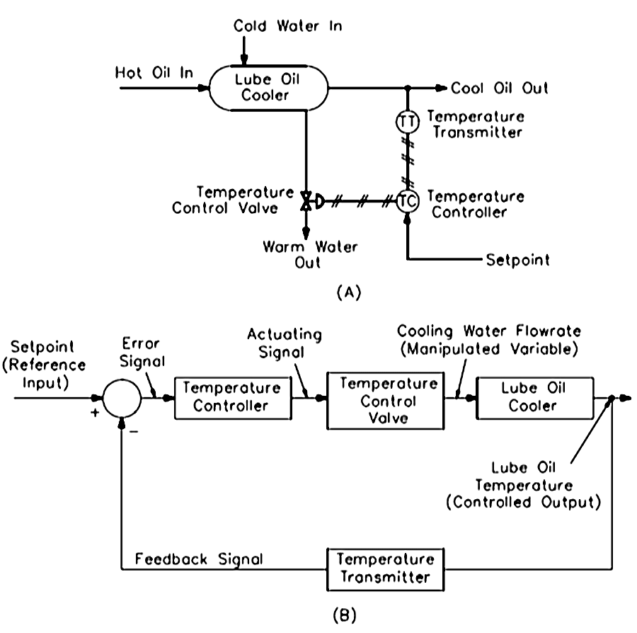
- The lube oil must be maintained within a specific operating band to ensure optimum equipment performance. This is accomplished by controlling the flow rate of the cooling water with a temperature control loop.
The temperature control loop consists of a temperature transmitter, a temperature controller, and a temperature control valve. The diagonally crossed lines indicate that the control signals are air (pneumatic).
The lube oil temperature is the controlled variable (output) because it is maintained at a desired value (the setpoint). Cooling water flow rate is the manipulated variable because it is adjusted by the temperature control valve to maintain the lube oil temperature.
- The temperature transmitter senses the temperature of the lube oil as it leaves the cooler and sends an air signal that is proportional to the temperature controller. Next, the temperature controller compares the actual temperature of the lube oil to the setpoint (the desired value).
If a difference exists between the actual and desired temperatures, the controller will vary the control air signal to the temperature control valve. This causes it to move in the direction and by the amount needed to correct the difference. For example, if the actual temperature is greater than the setpoint value, the controller will vary the control air signal and cause the valve to move in the open direction.
- (B) represents the lube oil temperature control loop in block diagram form. The lube oil cooler is the plant in this example, and its controlled output is the lube oil temperature. The temperature transmitter is the feedback element. It senses the controlled output and lube oil temperature and produces the feedback signal.
The feedback signal is sent to the summing point to be algebraically added to the reference input (the setpoint). Notice the setpoint signal is positive, and the feedback signal is negative. This means the resulting actuating signal is the difference between the setpoint and feedback signals.
The actuating signal passes through the two control elements: the temperature controller and the temperature control valve. The temperature control valve responds by adjusting the manipulated variable (the cooling water flow rate). The lube oil temperature changes in response to the different water flow rate, and the control loop is complete.
Components of a feedback control system (Cont.)
- Components: Disturbance signal
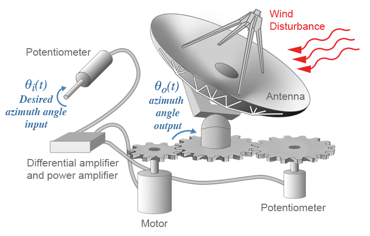
The disturbance is an undesirable input signal that upsets the value of the controlled output of the plant. For example consider the position control of an automatic satellite antenna system. An electrical motor is used to adjust the position of the antenna.
In this system the position of the satellite antenna is always subject to external forces such as the wind and air conditions.
In this system, wind is a disturbance signal which upsets the control system. In a well-designed control system, the output of the system is less sensitive to the disturbance changes.
Components: error signal
- This is the signal which actually drives the system. The error is the difference between the input and the measured output. This signal is calculated by the summing junction. Clearly when this signal is equal to zero, the output is reached to the desired value and tendency of the output to drift away from this value creates a nonzero error signal and the controller produces the appropriate response to minimise this error.A summing junction has only one output and is equal to the algebraic sum of the inputs.

-
Types of Control Systems and their response to standard test input signals
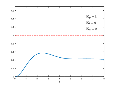
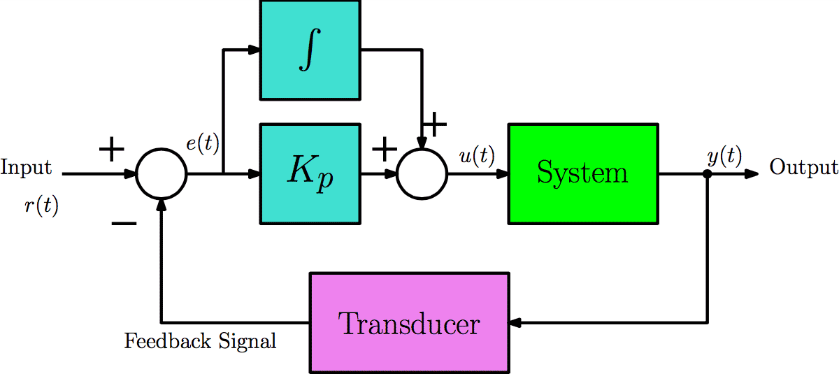
- Proportional Control System
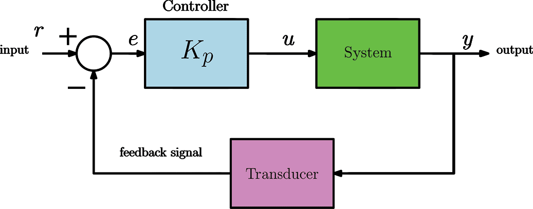
The performance of the control system can greatly change depending on the choice of controller. In this section we are going to learn about different controllers which are widely used in industry. The simplest controller is the proportional control system. In a proportional control system the controller is composed of an amplifier with a constant gain $K_p$. Therefore, the control signal applied to the system is $$ u=K_p\times e $$ Hence, the power supplied to the system (motor, robot arm, oven, chemical reactor etc.) will therefore be proportional to the tracking error signal, $e$
Proportional Control System
Step response of a system for different $K_p$ values: small $K_p$
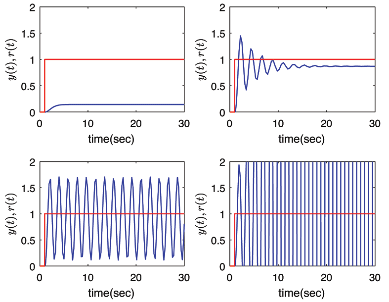
- In general the step response characteristics of a proportional control system is as follows: For very low values of $K_p$ the response is very sluggish and the required output is never reached (Top left). 📷 The below diagram can be seen larger here.
Continues on next tab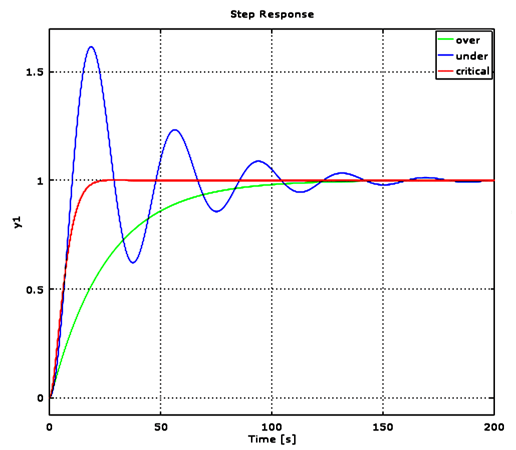
Performance parameters of control systems
- Test signals
Before we discuss the details of control systems and types of control, we need to define some metrics that would enable us to evaluate the performance of the control system. In order to define these metrics, we have to apply specific signals to the system and obtain the response of the system. These signals are called test signals. Although there are numerous signals that are used in control systems, in this course, we shall only use standard step input that is shown in figure. Please note that if a = 1 then the signal is called a unit step signal.

Step type test signal
- The input to the control system is suddenly increased from zero to another value a. This is an approach like closing a switch to suddenly apply a constant voltage a to the input. If the controlled system responds quickly to the above test signal and if the output settles to a value, then it should operate in the similar fashion with any other type of ”unknown or unexpected” input. If the system is stable the output will rise slowly until it settles to a constant value. A typical response is obtained as in the following figure:

Definitions
Rise Time: tr
The rise time is the time required for the response to rise from $10\%$ to $90\%$, $5\%$ to $95\%$, or $0\%$ to $100\%$ of its final value. For underdamped systems, the $0\%$ to $100\%$ rise time is normally used. For overdamped systems, the $10\%$ to $90\%$ rise time is commonly used.Settling Time: ts
Time it takes for the error $|y(t) - y_{final}|$ to fall to within $2\%$ or $5\%$ of $y_{final}$.Delay Time: td
The delay time is the time required for the response to reach half the final value the very first time.Peak Time: tp
The peak time is the time required for the response to reach the first peak of the overshoot.Maximum overshoot: Mp
The maximum overshoot is the maximum peak value of the response curve measured from unity. 📷 Response types graph seen here.
- Proportional Control System
-
How to use integral control?
- Integral control is rarely used on its own because the response of a pure integral control is generally very sluggish (big rise time). For this reason, integral controllers are usually combined with proportional controller, giving reasonable rise times with zero steady-state error. This type of control is known as Proportional+Integral Control (PI Control) and is shown in the following figure.
PI Controller
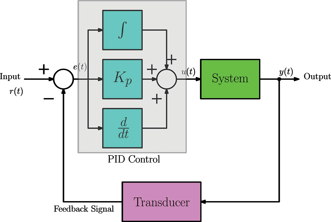
Differential Control Action and the PID Control
- Note
The performance of a PI controller is way better than the performance of a pure integral controller. The steady-state error which exists in a pure proportional control action does not exist anymore. However, the response is still slow. In order to decrease the rise time with a zero steady-state error we augment the PI control mechanism with differentiation which leads to the well-known Proportional+Integral+Derivative (PID) control
📷 The below diagram can be seen larger here.
Derivative action
How to use derivative control?
- Derivative control is never used on its own because it can generate very huge gains when the input changes fast. Especially when the input is rich of noise (signal having fast changes inside), the derivative action can be dangerous since it can generate huge signals at the output. Therefore, this type of control is used in combination with PI controllers which leads to PID control scheme.
Step response of a system for different $K_p$ values: normal level $K_p$
- As the gain is increased, rise time shortens and the steady state error decreases. But the overshoots starts to appear and the output oscillates (Top right).
📷 The below diagram can be seen larger here.
Step response of a system for different $K_p$ values: high level $K_p$
- As the gain is further increased, the rise time is very fast but the output oscillates continuously (Lower left). 📷 See lower left diagram - can be seen larger here.
Step response of a system for different $K_p$ values: very high level $K_p$
- When the controller gain is very high, the amplitude of the output oscillations increase and the system goes out of control which is nothing but called instability (Lower right). 📷 See lower right diagram - can be seen larger here.
Integral Control Action
- Moral of the story
In the light of results shown in previous slides, a pure proportional control cannot be used if the output must equal to the input. Which means that we are not able to clear the steady-state error. Also, for small tracking error we need to use high control gains which lead to huge overshoots and oscillations. Therefore we need other type of control mechanisms to overcome this situation. One approach is to add an integral action to the control.

- Working principle
A prime requirement of many systems is that there should be no error, or at worst a very small error in the steady-state. This can be achieved by replacing the proportional control gain, $K_p$ with an integral amplifier as shown above.In this case, even the smallest error will eventually produce a corrective control signal of sufficient magnitude to actuate the system to eliminate the tracking error due to the nature of integration.
📷 The below diagram can be seen larger here.
-
Simulation software
- In the following example we are going to design a P, PI and PID controller for a third order dynamic system. We shall use a tool developed by National Instruments to simulate the controller. Tool is free and can be downloadable from its website. This tool will allow you to run standalone LAbVIEW applications without installing LabView developer software. If you have LabVIEW developer software already installed on your computer then you do not need to install it and just skip step 1 and continue with step 2.
To install the required software please follow the following steps.
download the compressed file and extract it to an appropriate area in your machine. Then you are done! Just click on the tuner2015 application file and it must run.
Examples
- P Control - 1:
📷 Open P Control - 1
- P Control - 2:
📷 Open P Control - 2
- PI Control:
📷 Open PI Control
- PID Control:
📷 Open PID Control
Tuning PID controllers
- Ziegler-Nichols Tuning
As a result of emprical tests on a wide variety of process plant, Ziegler and Nichols proposed a simple rule of thumb procedure for estimating the controller gains $K_P$, $K_I$ and $K_D$ which are used to generate the control signal $$ u(t)=K_Pe(t)+K_I\int e(t)dt+K_D\frac{d}{dt}e(t) $$ where $e(t)$ is the error signal. Here, $K_P$ stands for the proportional gain; whereas, $K_I$ and $K_D$ stand for the integral and derivative control gains, respectively. Tuning process aims to find the optimal gains for $K_P$, $K_I$ and $K_D$.
- There are 2 different types of tuning technique for PID control. These are:
(a) Continuous cycling technique which is used on closed-loop systemsand:
(b) reaction curve technique which is used on open-loop systems.In this module we shall only consider continuous cycling method.
The general structure of a PID controller
- The general form of a PID controller is $$ u(t)=K\left[e(t)+\frac{1}{T_i}\int_0^te(\theta)\mathrm d\theta+T_d\frac{de(t)}{dt}\right] $$ where three parameters to tune are proportional control gain $K$; integral time constant, $T_i$ and the derivative time constant, $T_d$.
- It is easy to see that $K_p\equiv K$, $K_I\equiv \frac{K}{T_i}$ and $K_D\equiv KT_d$
Continuous cycling technique
- The goal is to find the best values of $K$, $T_i$ and $T_d$. The procedure is summarised as follows:
- Tuning algorithm:
Set $T_i=\infty$, $T_d=0$ which will disable the integrator and differentiator to make the system a pure proportional control systemSlowly increase the proportional gain $K$ until the system output is oscillatingMeasure the period $T_C$ of oscillations(in seconds) and record the gain that causes this oscillations. This value of $K$ is called the critical gain and denoted by $K_C$.Then the optimal values of PID controller are as follows:
► $K=0.5K_C$ for a proportional control system ( P)
► $K=0.4K_C$, $T_i=0.83T_C$ for a proportional+integral (PI) control system
► $K=0.6K_C$, $T_i=0.5T_C$ and $T_d=0.125T_C$ for a proportional+integral+derivative (PID) control system.
- We shall start with the design of a proportional controller (P) for the system having a transfer function $ G(s)=\large\frac{1}{s^3+3s^2+3s+1} $ where $s$ is the Laplace variable which stands for the time-derivative operation $d/dt$. According to this transfer function, the associated simulation screen should look like the following
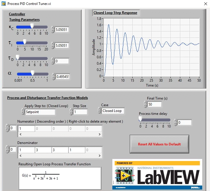 Here $\tau_I$ is the integral time constant $T_i$, $\tau_D$ is the derivative time constant $T_d$ and $K_C$ is the control gain $K$. Finally $\alpha$ stands for the derivative filter constant which needs to be tuned during the design.
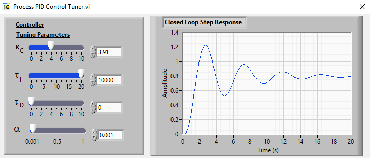
- Following the Ziegler-Nichols technique, the critical gain is found to be $K_C=7.83$ by setting $T_i=10000$, $T_d=0$. Hence, for the proportional control the control gain is found to be $K=3.91$ which gives the following system response. It is clear that the performance of the proportional control is very poor. The response is oscillatory and there is $25\%$ steady-state error, (set point=$1$, steady-state response=$0.75$)
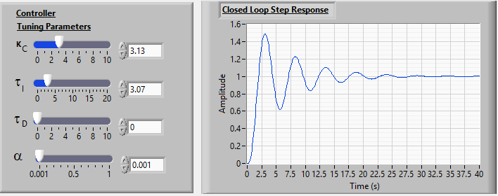
- Following the Ziegler-Nichols technique, the critical gain is found to be $K_C=7.83$ and the critical period, $T_C=3.7s$. Hence, for the proportional+integral control, the control gain and the integral constant are found to be as $K=3.13$ and $T_i=0.83\times 3.7=3.07 $ which give the following system response. It is clear that the performance of the PI control is very similar to the proportional controller but there is no steady-state error.
- Following the Ziegler-Nichols technique, the critical gain is found to be $K_C=7.83$ and the critical period, $T_C=3.7s$. Hence, for the proportional+integral control, the control gain, the integral constant and derivative constant are found to be as $K=4.7$ and $T_i=0.5\times 3.7=1.85$ and $T_d=0.125\times 3.7=0.46$ which give the following system response. It is clear that the performance of the PID control is much better than the PI and P controllers.

- In the following example we are going to design a P, PI and PID controller for a third order dynamic system. We shall use a tool developed by National Instruments to simulate the controller. Tool is free and can be downloadable from its website. This tool will allow you to run standalone LAbVIEW applications without installing LabView developer software. If you have LabVIEW developer software already installed on your computer then you do not need to install it and just skip step 1 and continue with step 2.