Week 1: Control and Instrumentation Systems

Wk 1

Control and Instrumentation Systems

Introduction and Motivation

Some Definitions: Signals and System

Instrumentation Systems

Performance of Measurement Systems

Example

Introduction and Motivation

To explain what a mechanical, electrical, chemical, or electrical engineer does is relatively easy, but it is another story to concisely describe the work performed by an engineer who specializes in instrumentation and control. Instrumentation and control are interdisciplinary fields. They require knowledge of chemistry, mechanics, electricity and magnetism, electronics, microcontrollers and microprocessors, software languages, process control, and even more such as the principles of pneumatics and hydraulics and communications. Control and instrumentation engineers (C&I engineers) are responsible for designing, developing, installing, managing and maintaining equipment which is used to monitor and control engineering systems, machinery and processes. Instrumentation and Control covers a range of topics which are important to the monitoring and control of modern systems. Instrumentation and control is a field applicable to many sectors of industry. It enables efficient and safe automatic control of large-scale continuous processes including nuclear power stations, oil refineries and chemical plants down to smaller batch operations such as manufacturing centres, breweries and other food production facilities.
Signal (cont.)

Signal processing involves the theory and application of filtering, coding, transmitting, estimating, detecting, analysing, recognizing, synthesizing, recording, and reproducing signals by digital or analog devices or techniques where signal includes audio, video, speech, image, communication, geophysical, sonar, radar, medical, musical, and other signals.

In mathematical sense, A signal is a function that maps an independent variable to a dependent variable. There are two types of signals: continuous-time signals and discrete-time signals. Continuous-time signals are functions of a continuous variable (time). Discrete-time signals are functions of a discrete variable; that is, they are de- fined only for integer values of the independent variable (time steps).

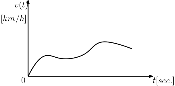
For example the speed of a car $ v(t) $ shown in Figure is a contiunous-time signal since the independent variable, time takes values from the set of real numbers which is continuous

However, the the signal $ x[n] $ , as shown below is a discrete-time signal because the signal has a value only for some specific time points.

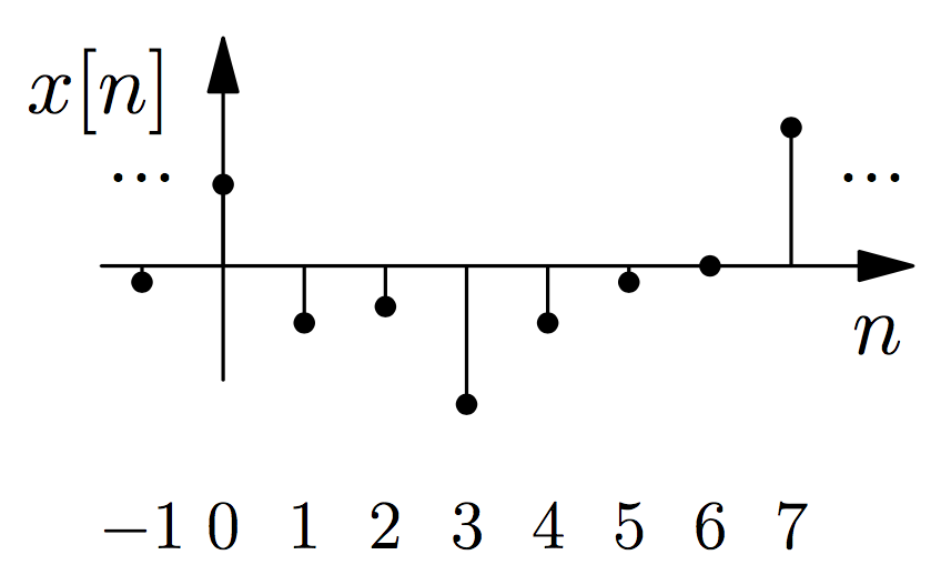
In a discrete-time signal $ x[n] $, the independent variable $ n $ is discrete (integer). To plot a discrete-time signal in a program like Matlab, you should use the stem or similar command and not the plot command

Definition: Instrumentation
An instrumentation system, also commonly known as measurement system, obtains data about a physical system either for the purpose of collecting information about that physical system or for the feedback control of the physical system. The term instrumentation may refer to something as simple as direct reading thermometers or, when using many sensors, may become part of a complex Industrial control system in such as manufacturing industry, vehicles and transportation. Instrumentation can be found in the household as well; a smoke detector or a heating thermostat are some simple examples from real life.

What is a measurement instrument?
A measurement instrument is a device capable of detecting change, physical or otherwise, in a particular process. It then converts these physical changes into some form of information understandable by the user. Consider the example of Figure 1.

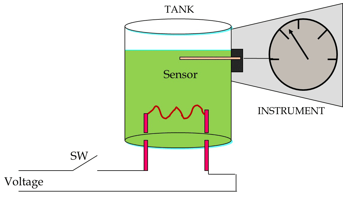
Figure 1: An example of a measurement instrument

– When the switch is closed, the resistor generates heat, increasing the temperature of the liquid in the tank. This increase is detected by the measurement instrument and shown on the scale of that instrument. We can get the information on the physical changes in a process using direct indication or a recorder.

Some Definitions: Signals and System

Signal
A signal is a detectable physical quantity by which messages or information can be transmitted. Examples:

– Speech signals transmit language via acoustic waves

– Radar signals transmit the position and velocity of targets via electromagnetic waves

– Electrophysiology signals transmit information about processes inside the body.

– Financial signals transmit information about events in the economy
(Cont.)
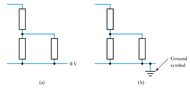
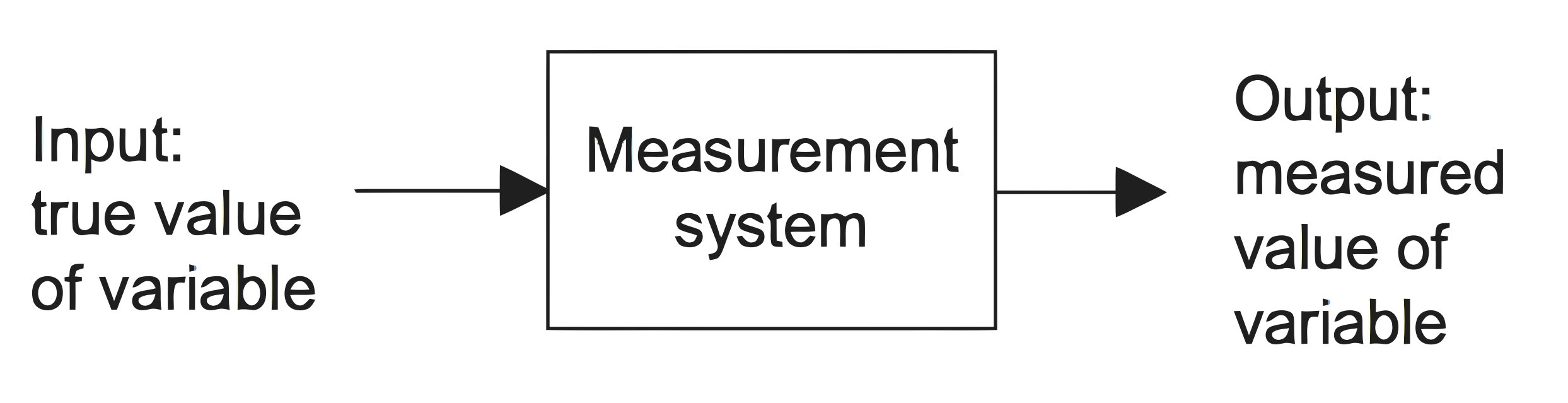
📷 An instrumentation system for making measurements has an input of the true value of the variable being measured and an output of the measured value. This output might be then used in a control system to control the variable to some set value. - as seen here.

Any instrumentation system must include an input device (sensor)(transducer) which measures the physical quantity such as speed, heat, pressure, height, position etc depending on the area where the device is used. This response to a particular stimulus mostly measured electrically. The other component that is generally present in modern instrumentation systems is a digital processor (controller), such as a computer, Digital Signal Processor (DSP) or a micro-controller. These programmable components have the flexibility to be used for a variety of functions and they can be reprogrammed easily using device-specific programming languages. The most important function that they perform is to convert physical data into information that can be used for computation and calculation. In the simplest situation the processing required to extract information may only involve converting an input signal by a scale factor so that the final result is in conventional units. For example, the output voltage signal from a strain gauge may be converted to the corresponding actual strain. Alternatively, within a more sophisticated system the signal from a strain gauge placed on an engine mounting might be processed to extract the vibrational spectrum of an engine, which is then used to detect any unusual frequency that might be indicative of wear. This information can then be displayed to a user, stored for later analysis, transmitted to a remote location or used by a controller.

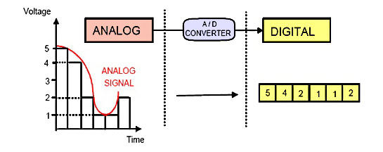
The signal received from sensor or measuring element is usually analogue in nature, ie. it is continuously varying with respect to an independent variable, time and can take any value (within an allowed range). This continuous analogue data has to be converted to a digital format prior to being transferred to the digital processor. Therefore, any instrumentation system must include an analogue-to-digital (A/D) converter (ADC for short) to convert this analogue signal into a digital format before processed by the computer.

The fundamental elements of an instrumentation system are sensor(s), computer (signal) processor(s) and data storage unit(s) / display device(s).

Some Definitions: Signals and System (cont.)

System manipulates the information carried by signals. It obtains data about a physical system either for the purpose of collecting information about that physical system or for the feedback control of the physical system.
A system can be defined as an arrangement of parts within some boundary which work together to provide some form of output from a specified input or inputs.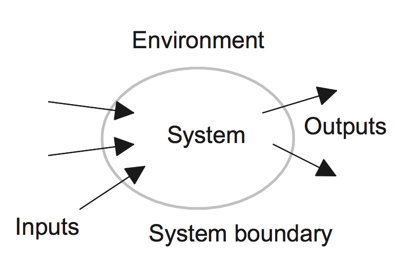
– The boundary divides the system from the environment.

– The system communicates with the environment by means of signals crossing the boundary from the environment to the system, called inputs, and signals crossing the boundary from the system to the environment, called outputs.

– A useful way of representing a system is as a block diagram. Within the boundary described by the box outline is the system, and inputs to the system are shown by arrows entering the box and outputs by arrows leaving the box.

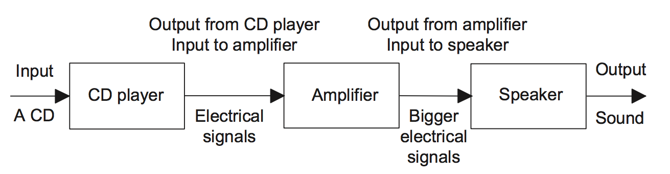
Often we are concerned with a number of linked systems. For example, we might have a CD player system linked to an amplifier system, which, in turn, is linked to a loudspeaker system. We can then draw this as three interconnected boxes with the output from one system becoming the input to the next system.

📷 In drawing a system as a series of interconnected blocks, it is necessary to recognise that the lines drawn to connect boxes indicate a flow of information in the direction indicated by the arrow and not necessarily physical connections - as seen here.

Instrumentation Systems

Also known as a measurement system, the purpose of an instrumentation system is to make measurements in order to give the user a numerical value corresponding to the variable being measured. Instrumentation is defined as the art and science of measurement and control of process variables within a production or manufacturing area. Instrumentation together with Control plays a significant role in both gathering information from the field and changing the field parameters, and as such are a key part of control loops.

Performance of Measurement Systems

Resolution is the smallest amount of an input signal change that can be reliably detected by an instrument. Resolution, as stated in a manufacturer’s specifications for an instrument is usually the degree to which a change can be theoretically detected, usually expressed as a number of bits. This relates the number of bits of resolution to the actual voltage measurements. For example, in order to determine the resolution of a system in terms of voltage, we have to make a few calculations. First, assume a measurement system capable of making measurements across a 10V range (20V span) using a 16-bits A/D converter. Next, determine the smallest possible increment we can detect at 16 bits. That is, $ 2^{16} = 65,536 $, or 1 part in 65,536, so $ 20V \div 65536 = 305\, \mu V $ per A/D count. Therefore, the smallest theoretical change we can detect is $ 305\, \mu \mathrm V $

Accuracy
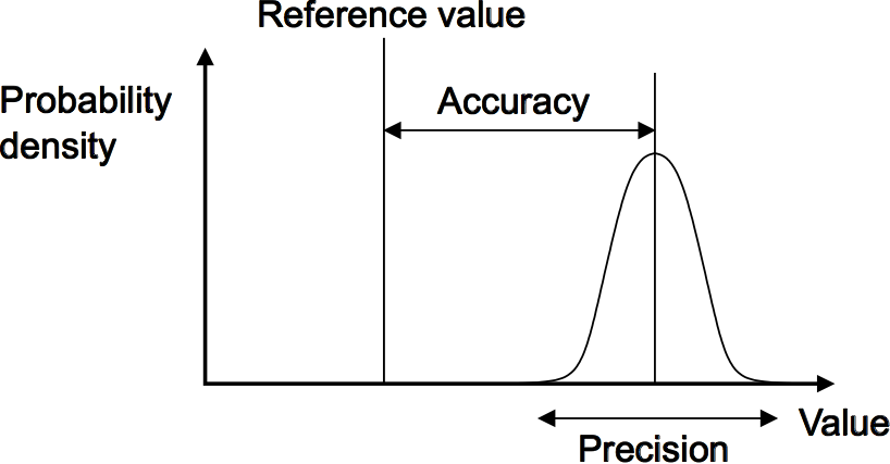
The closeness of a measurement to the actual value being measured. Also it is the extent to which the value indicated by a measurement system or element might be wrong. For example, a thermometer may have an accuracy of $ \pm 0.1 $. Accuracy is often expressed as a percentage of the full range output or full-scale deflection (f.s.d). For example, a system might have an accuracy of $ \pm 1\% $ of f.s.d. If the full-scale deflection is, say, 10A, then the accuracy is $ \pm 0.1 $A.

Error is used for the difference between the result of the measurement and the true value of the quantity being measured, i.e. Error = Measured Value - True Value Thus, for example, if the measured value is 9.1 when the true value is 9.0, the error is 0.1. Errors can arise in a number of ways and the following describes some of the errors that are encountered in specifications of instrumentation systems:

Hysteresis error:
The term hysteresis error is used for the difference in outputs given from the same value of quantity being measured according to whether that value has been reached by a continuously increasing change or a continuously decreasing change. For example, you might obtain a different value from a thermometer used to measure the same temperature of a liquid if it is reached by the liquid warming up to the measured temperature or it is reached by the liquid cooling down to the measured temperature.

💡MINI QUIZ

Instrumentation Systems (cont.)

Sensor
In the broadest definition, a sensor is an electro-mechanical, mechanical or electronic component, module, or subsystem whose purpose is to detect events or changes in its environment and send the information to other electronics, frequently a computer(signal) processor.
A good sensor obeys the following rules:

– it is sensitive to the measured property

– it has a linear transfer function (input-output relation)

– it is insensitive to any other property likely to be encountered in its application

– it does not influence the measured property.

Computer (signal) processor
This element takes the output from the sensor and converts it into a form which is suitable for display or storage.

Data Storage Unit(s) / Display Device(s)
This presents the measured value in a form which enables an observer to recognise it. This may be via a display, e.g. a pointer moving across the scale of a meter or perhaps information on a visual display unit (VDU). Alternatively, or additionally, the signal may be recorded, e.g. in a computer memory, or transmitted to some other system such as a control system. This presents the measured value in a form which enables an observer to recognise it. This may be via a display, $ \textit{e.g.} $ a pointer moving across the scale of a meter or perhaps information on a visual display unit (VDU). Alternatively, or additionally, the signal may be recorded, e.g. in a computer memory, or transmitted to some other system such as a control system.

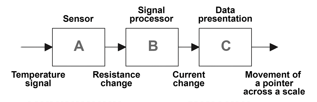
Example: A temperature measurement system
With a resistance thermometer, a sensor is used to measure the actual temperature which produces a resistance change depending on the temperature in the environment; a signal processor is used to transform the change in the value of resistance into a change in the current.

📷 Finally, a data presentation mechanism is used to transform the current signal into a display of a movement of a pointer across a scale. - as seen here.

Question #1 - Hysteresis error depends on the history of signal? False True	Question #2 - A good sensor does not influence the measured property . False True

The ‘average’ represents the mean of a series of numbers. It does not give any indication of the spread of these numbers. For example, suppose eight different voltmeter readings are taken of a fixed voltage, and the values read are 97, 98, 99, 100, 101, 102, 103 V. Hence, the mean value will be 100 V. If the readings are changed to 90, 90, 95, 100, 100, 105, 110, 110, the mean will still be 100

V, although now they are more widely separated from the mean. The three techniques most frequently used to measure dispersion from the mean are the range, mean deviation and the standard deviation.

The mean deviation, $ M $, is found by taking the mean of the difference between each individual number in the series and the arithmetic mean, and ignoring negative signs. Therefore for a series of $ n $ numbers $ x_1,x_2,\ldots,x_n $, having an arithmetic mean $ \bar x $, the mean deviation is given by $$ \large M=\frac{\sum_{r=1}^n|x_r-\bar x|}{n} $$
For the first set of values, the mean deviation is $ M=1.50 $V; and for the second set of values, the mean deviation is $ M=6.50 $V. Therefore, by comparing the mean deviation of the two sets of readings, one can deduce that the first set is more closely clustered around the mean, and therefore represents more consistent values. Neither the mean deviation nor the range are suitable for use in statistical calculation. The standard deviation is the measure of dispersion that is most commonly used for this. The standard deviation of a series of n numbers $ x_1,x_2,\ldots,x_n $ , having an arithmetic mean $ \bar x $ is given by $$ \large \sigma=\left (\frac{\sum_{r=1}^n(x_r-\bar x)^2}{n}\right )^{1/2} $$

Range
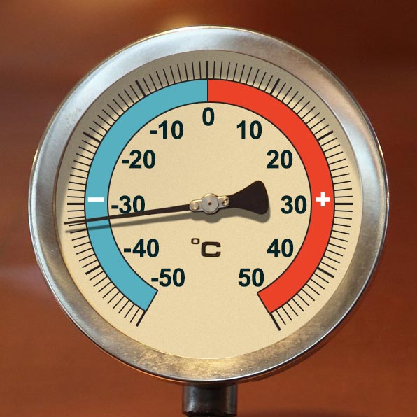
The range of variable of system is the limits between which the input can vary. It can be defined as the measure of the instrument between the lowest and highest readings it can measure. On the thermometer below the scale is from -50°C to +50°C. Thus the range varies from -50°C to +50°C.

Performance of Measurement Systems (cont.)

Nonlinearity error:
The term non-linearity error is used for the error that occurs as a result of assuming a linear relationship between the input and output over the working range, i.e. a graph of output plotted against input is assumed to give a straight line.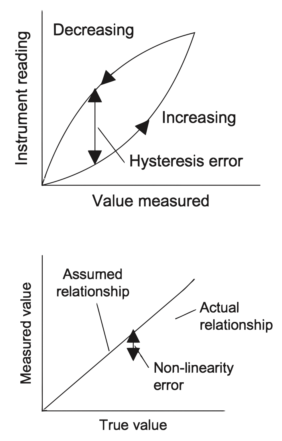

Insertion / Loading error:
When a cold thermometer is put in to a hot liquid to measure its temperature, the presence of the cold thermometer in the hot liquid changes the temperature of the liquid. The liquid cools and so the thermometer ends up measuring a lower temperature than that which existed before the thermometer was introduced. The act of attempting to make the measurement has modified the temperature being measured. This effect is called loading and the consequence as an insertion error. Loading is a problem that is often encountered when measurements are being made. For example, when an ammeter is inserted into a circuit to make a measurement of the circuit current, it changes the resistance of the circuit and so changes the current being measured.
Statistical analysis is frequently used in measurements and error analysis and the following mathematical concepts are widely used in measurements:

Average
The most frequently used averaging technique is the ‘arithmetic mean’. If $ n $ readings are taken with an instrument, and the values obtained are $ x_1,x_2,\ldots,x_n $ then the arithmetic mean is $$ \large \bar x=\frac{\sum_{r=1}^nx_r}{n} $$ Although the arithmetic mean is easy to calculate it is influenced unduly by extreme values, which could be false. An alternative averaging technique, called the geometric mean, is not overly affected by extreme values. It is often used to find the average of quantities that follow a geometric progression or an exponential law. The geometric mean is given by $$ \large x_g=(x_1 \times x_2 \times \cdots \times x_n)^{1/n} $$

Sensitivity
The sensitivity indicates how much the output of an instrument system or system element changes when the quantity being measured changes by a given amount, i.e. the ratio output/input. For example, a thermocouple might have a sensitivity of $20 \mu V/C$ and so give an output of $20\, \mu \mathrm V$ for each 1°C change in temperature. Thus, if we take a series of readings of the output of an instrument for a number of different inputs and plot a graph of output against input, the sensitivity is the slope of the graph.

Stability and Drift
Stability of a system is its ability to give the same output when used to measure a constant input over a period of time. The term drift is often used to describe the change in output that occurs over time. The drift may be expressed as a percentage of the full range output. The The term zero drift is used for the changes that occur in output when there is zero input. Dead band/time The dead band sometimes known as dead space of a transducer is the range of input values for which there is no output. For example, bearing friction in a flow meter using a rotor might mean that there is no output until the input has reached a particular velocity threshold. The dead time is the length of time from the application of an input until the output begins to respond and change.

Dead band/time
The dead band sometimes known as dead space of a transducer is the range of input values for which there is no output. For example, bearing friction in a flow meter using a rotor might mean that there is no output until the input has reached a particular velocity threshold. The dead time is the length of time from the application of an input until the output begins to respond and change.

💡MINI QUIZ

Performance of Measurement Systems (cont.)

Precision
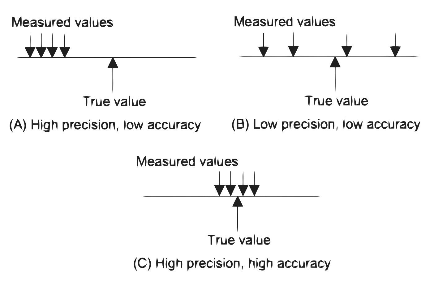
Precision is the fineness to which an instrument can be read repeatably and reliably. The term precision is used to describe the degree of freedom of a measurement system from random errors. Thus, a high precision measurement instrument will give only a small spread of readings if repeated readings are taken of the same quantity. A low precision measurement system will give a large spread of readings.

📷 For example, consider the following two sets of readings obtained for repeated measurements of the same quantity by two different instruments:
The results of the measurement give values scattered about some value. The first set of results shows a smaller spread of readings than the second and indicates a higher degree of precision for the instrument used for the first set.

Question #1 - High Precision Instrument is the same as Accurate Instrument: True False	Question #2 - High Precision Instrument can have significant Error: True False

**2 Sets of Reading obtained by 2 different measurement devices of the same quality**
Instrument 1	20.1mm	20.2mm	20.0mm	20.1mm	20.1mm	20.1mm	20.0mm
Instrument 2	19.9mm	20.3mm	20.0mm	20.5mm	20.2mm	19.8mm	20.3mm

Repeatability
Repeatability is used for the ability of a measurement system to give the same value for repeated measurements of the same value of a variable. Common causes of lack of repeatability are random fluctuations in the environment, e.g. changes in temperature and humidity. The error arising from repeatability is usually expressed as a percentage of the full range output. For example, a pressure sensor might be quoted as having a repeatability of ±0.1% of full range. Thus with a range of 20 kPa, that would be an error of ±20 Pa.

Reproducibility is used describe the ability of a system to give the same output when used with a constant input with the system or elements of the system being disconnected from its input and then reinstalled. The resulting error is usually expressed as a percentage of the full range output.
Note: The precision should not be confused with accuracy. High precision does not mean high accuracy. A high precision instrument could have low accuracy.

(Cont.)

Peak time ($ t_p $) is the time required for the response to reach the first peak of the overshoot.
Maximum (percent) overshoot ($ M_p $)The maximum overshoot is the maximum peak value of the response curve measured from unity. If the final steady-state value of the response differs from unity, then it is common to use the maximum percent overshoot. It is defined by $$ \large M_p=\frac {y(t_p)-y(\infty)}{y(\infty)}\times 100 $$ Settling time $ (ts) $ is the time required for the response curve to reach and stay within a range about the final value of size specified by absolute percentage of the final value (usually $ 2\% $ or $ 5\% $ ). The settling time is related to the largest time constant of the control system.
The Rubik's Cube solver runs in your web browser and it finds the solution for your puzzle in seconds.

Example

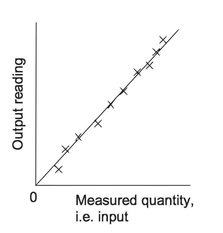
📷 Question - A spring balance has its deflection measured for a number of loads and gave the following results - seen here. Determine its sensitivity.

📷 Answer - The figure here shows the graph of output against input.

**2 Sets of Reading obtained by 2 different measurement devices of the same quality**
Load in kg	0	1	2	3	4
Deflection in mm	0	10	20	30	40

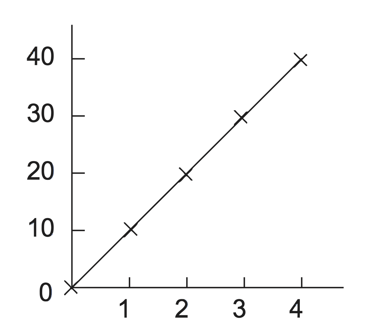Since the graph has a slope of 10 mm/kg, the sensitivity is 10.

Performance of Measurement Systems (cont.)

Dynamic (Transient) Characteristics of the Instrument
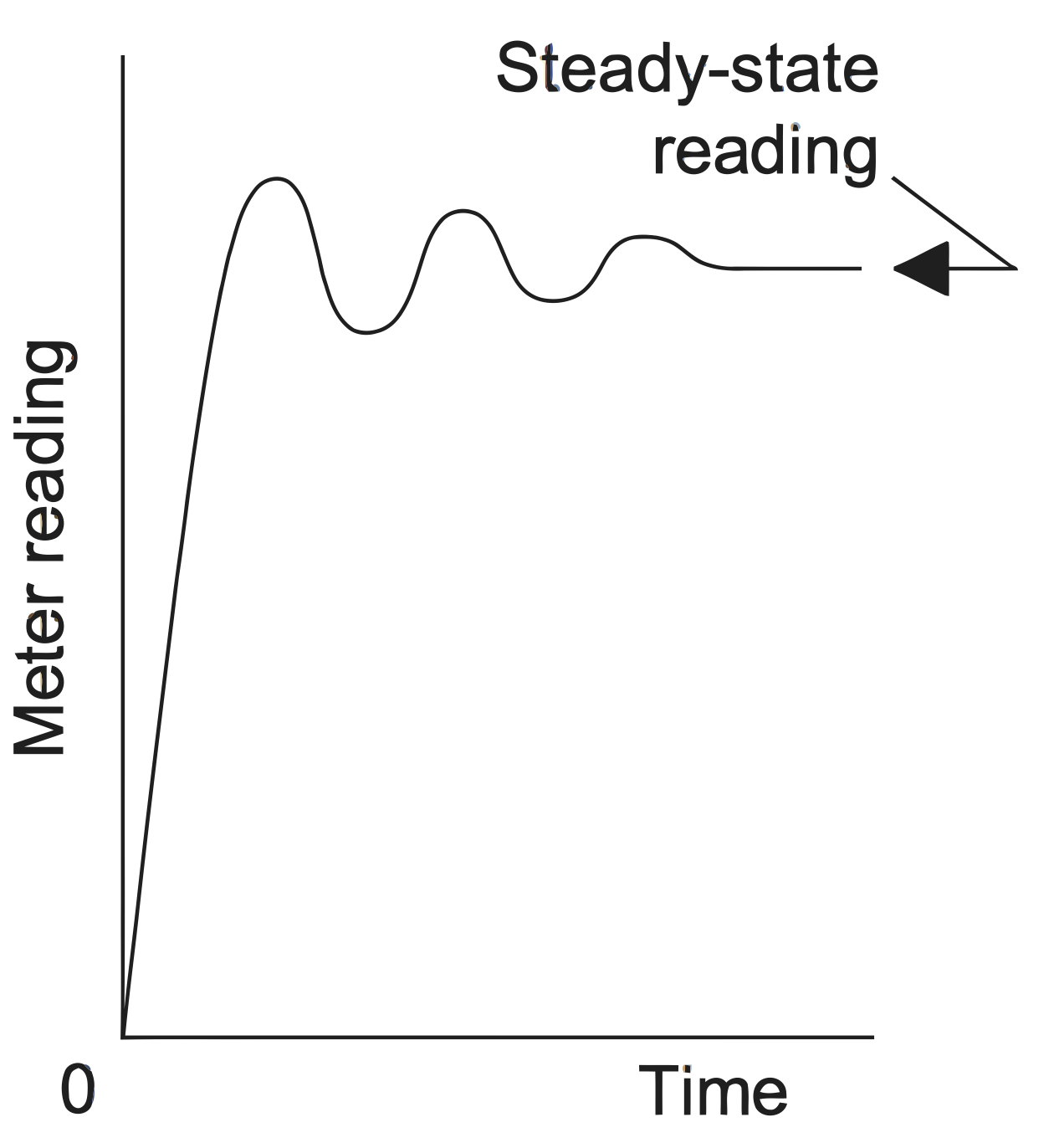
The terms that we have discussed so far refer to what can be termed the static characteristics. These are the values given when steady-state conditions occur, i.e. the values given when the system or element has settled down after having received some input. The dynamic (transient) characteristics refer to the behaviour between the time that the input value changes and the time that the value given by the system or element settles down to the steady-state value. For example, the following figure shows how the reading of an analogue ammeter might change when the current is switched on. The meter pointer oscillates before settling down to give the steady-state reading. A typical transient response is in the form of the following figure:

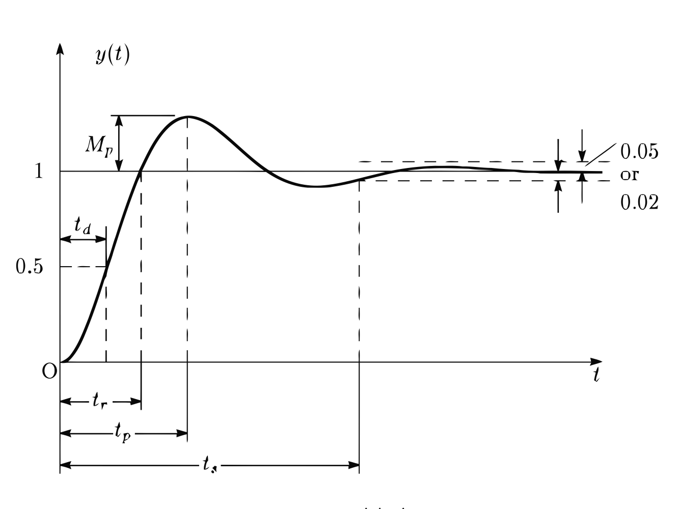
Delay time $ (td) $ is the time required for the response to reach half the final value the very first time.
Rise time $ (tr) $ is the time required for the response to rise from $ 10\% $ to $ 90\% $, $ 5\% $ to $ 95\% $, or $ 0\% $ to $ 100\% $ of its final value. For underdamped second-order systems, the $ 0\% $ to $ 100\% $ rise time is normally used. For overdamped systems and the systems which have dead-zone, the $ 10\% $ to $ 90\% $ rise time is commonly used.