Week 3: Control and Instrumentation Systems

Wk 3

Displacement, proximity and shift sensors
A displacement, proximity or shift sensor is here considered to be one that can be used to:

1. Measure a linear displacement, i.e. a change in linear position. This might, for example, be the change in linear displacement of a sensor as a result of a change in the thickness of sheet metal emerging from rollers.

2. Measure an angular displacement, i.e. a change in angular position. This might, for example, be the change in angular displacement of a drive shaft.

3. Detect motion, e.g. this might be as part of an alarm or automatic light system, whereby an alarm is sounded or a light switched on when there is some movement of an object within the ‘view’ of the sensor.

4. Detect the presence of some object, i.e. a proximity sensor. This might be in an automatic machining system where a tool is activated when the presence of a work piece is sensed as being in position.

Displacement sensors fall into two groups: those that make direct contact with the object being monitored, by spring loading or mechanical connection with the object, and those which are non-contacting. For those linear displacement methods involving contact, there is usually a sensing shaft which is in direct contact with the object being monitored, the displacement of this shaft is then being monitored by a sensor. This shaft movement may be used to cause changes in electrical voltage, resistance, capacitance, or mutual inductance. For angular displacement methods involving mechanical connection, the rotation of a shaft might directly drive, through gears, the rotation of the sensor element, this perhaps generating an e.m.f. Non-contacting proximity sensors might consist of a beam of infrared light being broken by the presence of the object being monitored, the sensor then giving a voltage signal indicating the breaking of the beam, or perhaps the beam being reflected from the object being monitored, the sensor giving a voltage indicating that the reflected beam has been detected. Contacting proximity sensors might be just mechanical switches which are tripped by the presence of the object, the term limit switch being used. The following are examples of displacement sensors.

Capacitance Transducers

The capacitance C of a parallel plate capacitor (Figure 3) is given by:
$$𝐶=\frac{\varepsilon _0 \varepsilon _r}{d}A$$ where $\varepsilon $_r is the relative permittivity of the dielectric between the plates, $\varepsilon $₀ a constant called the permittivity of free space (=8.85x10^-12F/m)¹, A the area of overlap between the two plates and d the plate separation. The capacitance will change if the plate separation $d$ changes, the area $A$ of overlap of the plates changes, or a slab of dielectric is moved into or out of the plates, so varying the effective value of $εr$ (Figure 4). All these methods can be used to give linear displacement sensors.

Figure 3. Parallel plate

Figure 4. Capacitive sensors

Capacitive Transducers using Change in Distance Between Plates
Figure 5. Illustrates typical arrangement of a capacitance transducer that employs plate distance variations causing change in capacitance. The right plate is fixed, and the left plate is movable by the displacement, which is to be measured. The capacitance is computed as: $$𝐶=\frac{\varepsilon _0 \varepsilon _r}{d}A$$

Figure 5. Capacitance change due to plate separation

Note: F is symbol for Farad, SI derived unit for electrical capacitance

If air is the dielectric medium, $\varepsilon $_r$=1$. The capacitance is inversely proportional to the distance between plates. The overall response of the transducer is not linear, as shown by the distance versus capacitance plot of Figure 6; hovewer, transducer of this type are used for the measurement of extremely small displacements, where the relationship is approximately linear: $$ S= \frac {\partial C}{\partial d} = \frac{^- \varepsilon _0 \varepsilon _r}{d ^2} A $$

Figure 6. Variation of capacitance with distance

💡MINI QUIZ

Continues on next tab

Potentiometer

A potentiometer consists of a resistance element with a sliding contact which can be moved over the length of the element and connected as shown in 1. With a constant supply voltage Vs, the output voltage V_o between terminals 1 and 2 is a fraction of the input voltage, the fraction depending on the ratio of the resistance R₁₂ between terminals 1 and 2 compared with the total resistance R of the entire length of the track across which the supply voltage is connected. Thus V_o/V_s=R₁₂/R. If the track has a constant resistance per unit length, the output is proportional to the displacement of the slider from position 1. A rotary potentiometer consists of a coil of wire wrapped round into a circular track, or a circular film of conductive plastic or a ceramic-metal mix termed a cermet, over which a rotatable sliding contact can be rotated. Hence an angular displacement can be converted into a potential difference. Linear tracks can be used for linear displacements.

Figure 1 Potentiometer

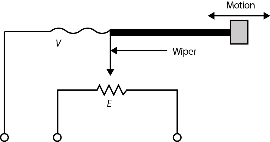
Figure 2 Principle of the potentiometer transducer

Figure 2 shows how the voltage across the wiper of linear potentiometer is measured in terms of the displacement $d$, and given by the relationship:
$$ V = E\frac{d}{L}$$ Here $E$ is the voltage across potentiometer, and $L$ is the full-scale displacement of the potentiometer.
With a wire-wound track the output voltage does not continuously vary as the slider is moved over the track but goes in small jumps as the slider moves from one turn of wire to the next. This problem does not occur with a conductive plastic or the cermet track. Thus, the smallest change in displacement which will give rise to a change in output, i.e. the resolution, tends to be much smaller for plastic tracks than wire-wound tracks. Errors due to non-linearity of the track for wire tracks tend to range from less than $0.1%$ to about $1%$ of the full range output and for conductive plastics can be as low as about $0.05%$.
The track resistance for wire-wound potentiometers tends to range from about $20 Ω$ to $200 kΩ$ and for conductive plastic from about $500 Ω$ to $80 kΩ$.

Conductive plastic has a higher temperature coefficient of resistance than wire and so temperature changes have a greater effect on accuracy. The resolution of such a sensor depends on its construction. If it is a wire-wound coil with a rotatable sliding contact then the finer the wire the higher the resolution. Thus a sensor with $25$ turns per mm would have a resolution of $640 μm$. Such a sensor has a fast response time and a low cost.

An application of a potentiometer is to sense the position of the accelerator position in an automobile and feed the information to the engine control system. Another potentiometer might be used as the throttle position sensor.

Question #1 - What is a potentiometer: Instrument for measuring of electrical potential Variable resistor Capacitance sensor	Question #2 - Potentiometers are non-contact sensors: False True

Cylindrical Capacitance Transducers
Concentrical Cylindrical Capacitors are often more convenient than Parallel Plates (Figure10)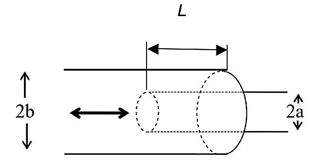
Figure 10. Cylindrical Capacitance Transducer

The capacitance is computed as: $$ C= \frac{2 \pi \varepsilon _r \varepsilon _0 L}{ln \frac{b}{a}} $$ This formula shows that the capacitance are linearly proportional to both, length $L$, and the relative dielectric constant $\varepsilon _r$, and varying any of them will produce the change in capacitance, therefore, in an analogous way to two-plate capacitance we can use this property for displacement measurement.
📷 Figure 11 shows how cylindrical capacitance transducer can be used as a level sensor for a dielectric liquid.

Capacitance Transducers based on Differential Arrangement
Differential capacitance transducers are also used for precision displacement measurement.
📷 Figure 12 shows two fixed plates and movable plate to which displacement is applied Let $C _1$ and $C _2$ be the capacitances of two plates which are fixed. Plate m is midway between the two plates. An alternating voltage, E, is applied across the plates, $P _1$ and $P _2$, and the potential differences across the two capacitors is measured. Assuming $ \varepsilon = \varepsilon _0 \varepsilon _r $ the following equations are written: $$ C _1 = \frac{\varepsilon A}{d}, \quad C _2 = \frac{\varepsilon A}{d} $$ Voltage across C1: $$ E _1 = \frac{EC _2}{C _1 + C _2} = \frac{E}{2} $$ And across C2: $$ E _2 = \frac{EC _1}{C _1 + C _2} = \frac{E}{2} $$ At midway point, $E _1- E _2$ is zero. If x is displacement of movable plate, then we have: $$ C _1 = \frac{\varepsilon A}{d + x}, \quad C _2 = \frac{\varepsilon A}{d - x} $$ he differential output voltage is $$ \Delta E - E _1 - E _2 = \frac{d + x}{2 d} E - \frac{d - x}{2 d} E = \frac{x}{d} E $$ The output voltage varies linearly with displacement $x$. Capacitance transducers based on differential arrangement are used for measurement applications in the range of 0.001 to 10mm and provide accuracy up to 0.05%. The sensitivity of the transducer is $$ S = \frac{\Delta E}{x} = \frac{E}{d}$$ A capacitive transducers have several advantages. They require extremely small forces to operate, are very sensitive and require low power to operate. Their frequency response is good up to 50kHz, making them good candidates for applications involving dynamics. Disadvantages include need to insulate metallic parts from each other and loss of sensitivity due to error sources associated with the cable connecting transducer to the measuring point.
Non-linearity and hysteresis error ±0.01% of full range

Capacitance Transducers (Cont.)

Capacitance Transducers using Change in Area of Plates
For parallel plate capacitors, the capacitance is given by: $$ C=\frac{\varepsilon _0 \varepsilon _r A}{d} = \frac{\varepsilon _0 \varepsilon _r Lw}{d} $$ Where $L$ is the lengths of overlapping parts of plates, and w the width of the overlapping parts (Figure 7)

Figure 7. Capacitance change due to change of area between plates

The sensitivity of the capacitance transducers becomes: $$ S= \frac {\partial C}{\partial l} = \frac{\varepsilon _0 \varepsilon _r Lw}{d}$$ There is linear relationship between displacement and the capacitance. This equation show that the capacitance is directly proportional to the area of the overlapping plates and varies linearly with the changes in the displacement between plates. Transducers of this type are convenient for measuring of relatively large displacements. (Figure 8)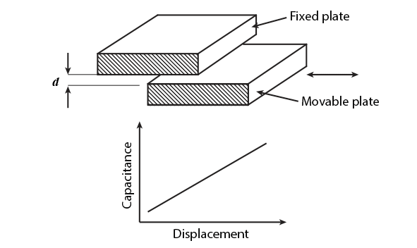
Figure 8. Capacitance change due to the variation of overlapping area

Capacitance Transducers using Variations of Dielectric Constant
The change in capacitance caused by a change the dielectric constant of the separating material is another principle which can be used in capacitance transducers. Figure 9 shows an arrangement of two plates separated by a material of different dielectric constant. As this material is moved, it causes a variation of dielectric constant in the region separating the two electrodes, resulting in change in capacitance.

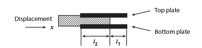Figure 9. Capacitance transducers using Variations of Dielectric Constant

The initial value of the capacitance, assuming a dielectric material of thickness $d$ and width $w$ can be described as: $$ C=\frac{\varepsilon _0 wl_1}{d} + \frac{\varepsilon _0 \varepsilon r wl_2}{d} = \frac{\varepsilon _0 w}{d} (l_1 + \varepsilon _rl_2) $$ This equation has two terms. One represents capacitance of the two electrodes separated by air, and the other represents capacitance of the dielectric material between the electrodes. If the dielectric material is moved through a distance x, as shown in Figure 9, the capacitance increases from $C$ to $C+\Delta C$, and the change in capacitance is equal to: $$C + \Delta C = \frac{ \varepsilon _0 w}{d} \{l1 - x + \varepsilon _r(l_2 + x)\}$$ $$C + \Delta C = \frac{ \varepsilon _0 w}{d} \{l1 + \varepsilon _rl_2 - x(\varepsilon _r - 1)\}$$ $$ \Delta C = \frac{\varepsilon _0 wx (\varepsilon _r - 1}{d} $$ The change in capacitance is linearly proportional to the displacement $x$.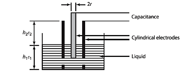

Figure 11. Cylindrical Capacitance Level sensor for a dielectric liquid

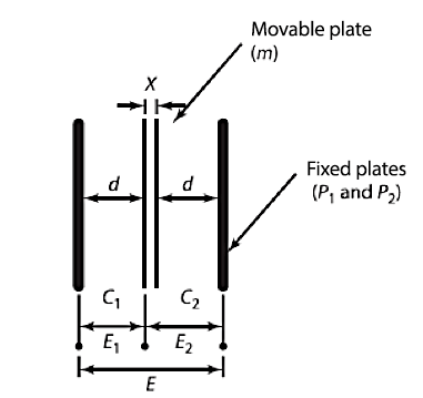
Figure 12. Differential arrangement of plates

Figure: Output Module
(Cont.)
With the incremental encoder, the number of pulses counted gives the angular displacement, a displacement of, say, 50° giving the same number of pulses whatever angular position the shaft starts its rotation from. However, the absolute encoder gives an output in the form of a binary number of several digits, each such number representing a particular angular position.
📷 Figure 15 here shows the basic form of an absolute encoder for the measurement of angular position.
With the form shown in the figure, the rotating disc has four concentric circles of slots and four sensors to detect the light pulses. The slots are arranged in such a way that the sequential output from the sensors is a number in the binary code, each such number corresponding to a particular angular position. A number of forms of binary code are used. Typical encoders tend to have up to 10 or 12 tracks. The number of bits in the binary number will be equal to the number of tracks. Thus with 10 tracks there will be 10 bits and so the number of positions that can be detected is 2¹⁰, i.e. 1024, a resolution of 360/1024 = 0.35°.
The incremental encoder and the absolute encoder can be used with linear displacements if the linear displacement is first converted to a rotary motion by means of a tracking wheel (Figure 16).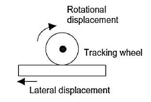

Figure 16. Tracking wheel

Linear encoder (Reflection type)
One of the possible use of optical gratings in linear form and using reflection is shown in Figure 17. In this the light must pass to the scale grating through the index grating and be reflected back through the index grating again to the photoelectric sensor. The fixed portion of the transducer box consists of a source of light, associated optics, and the detection system. The output of the detector is shown in the form of a digital read out. These types of transducers are popular in the machine-tool industry.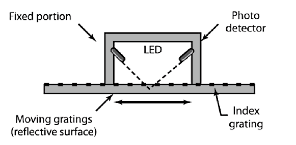

Figure 17. Linear encoder, reflection type

Moiré fringes are produced when light passes through two gratings which have rulings inclined at a slight angle to each other. Movement of one grating relative to the other causes the fringes to move.
📷 Figure 18(A) (seen here) illustrates this. Figure 18(B) shows a transmission form of instrument using Moiré fringes and Figure 18(C) a reflection form.

Moire Pattern Videos - view fullscreen

📷 In Figure 19 (seen here) there are a variety of optical sensors that can be used to determine whether an object is present or not. Figure 20 (below) shows an example of such a sensor (Pyroelectric sensor shown in the above link). Such sensors can be used with burglar alarms or for the automatic switching on of a light when someone walks up the drive to a house. A special lens is put in front of the detector. When an object which emits infrared radiation is in front of the detector, the radiation is focused by the lens onto the detector. But only for beams of radiation in certain directions will a focused beam fall on the detector and give a signal. Thus when the object moves then the focused beam of radiation is effectively switched on and off as the object cuts across the lines at which its radiation will be detected. Thus the pyroelectric detector gives a voltage output related to the changes in the signal.
Figure 20. Pyroelectric sensor

Figure 18(A) illustrates this. Figure 18(B) shows a transmission form of instrument using Moiré fringes and Figure 18(C) a reflection form.
With both, a long grating is fixed to the object being displaced. With the transmission form, light passes through the long grating and then a smaller fixed grating, the transmitted light being detected by a photocell. With the reflection form, light is reflected from the long grating through a smaller fixed grating and onto a photocell. Coarse grating instruments might have 10 to 40 lines per millimetre, fine gratings as many as 400 per millimetre. Movement of the long grating relative to the fixed short grating results in fringes moving across the view of the photocell and thus the output of the cell is a sequence of pulses which can be counted. The displacement is thus proportional to the number of pulses counted. Displacements as small as 1 μm can be detected by this means. Such methods have high reliability and are often used for the control of machine tools.

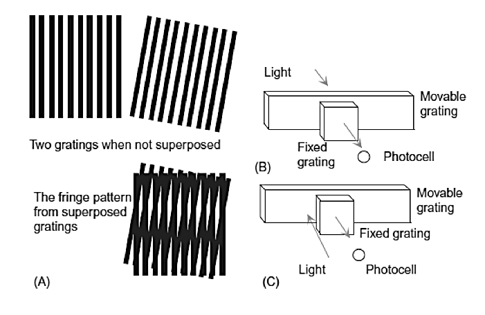
Figure 18 (A) Moiré fringes, (B) transmission, and(C) reflection forms of instrument.

Optical Proximity Sensors

There are a variety of optical sensors that can be used to determine whether an object is present or not. Photoelectric switch devices can either operate as transmissive types where the object being detected breaks a beam of light, usually infrared radiation, and stops it reaching the detector (Figure 19(A)) or reflective types where the object being detected reflects a beam of light onto the detector (Figure 19(B)).
In both types the radiation emitter is generally a light-emitting diode (LED). The LED is a basic pn junction diode which emits light when suitable voltage is applied to it. The LED emits radiation which is reflected by the object. The reflected radiation is then detected by a phototransistor. In the absence of the object there is no detected reflected radiation; when the object is in the proximity, there is. The radiation detector might be a photodiode or a phototransistor, often a pair of transistors, known as a Darlington pair; using the pair increases the sensitivity.
Depending on the circuit used, the output can be made to switch to either high or low when light strikes the transistor. Such sensors are supplied as packages for sensing the presence of objects at close range, typically at less than about 5 mm.

Figure 19(C) shows a U-shaped form where the object breaks the light beam and so changes the response from a photodetector.

Another form of optical sensor is the pyroelectric sensor. Such sensors give a voltage signal when the infrared radiation falling on them changes, no signal being given for constant radiation levels. Lithium tantalate is a widely used pyroelectric material.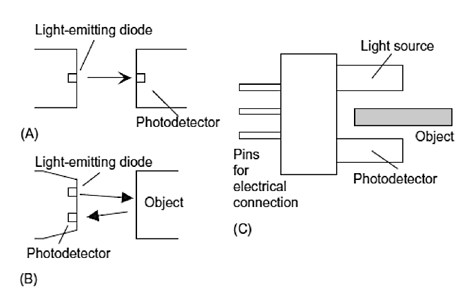

Figure 19. Photoelectric proximity sensors

Example 1: Normally Open Contacts

Figure shows a practical example which uses normally open contacts in the ladder diagram

When the switch is closed, $+24V$ is connected to IN1 of the PLC. This closes the contacts IN1 of the ladder diagram to energise control relay RC1 and hence turn load ON.

If the switch is opened again, the contacts IN1 will spring open de-energising relay RC1 turning load OFF.

Figure: Normally Open contacts: The input contacts (IN1 etc) are not real contacts, they are part of the program.

Example 2: Normally Closed Contacts

Figure shows a practical example which uses normally closed contacts in the ladder diagram

Initially control relay RC1 is energised through normally closed contacts IN1.

When the switch is closed, contacts IN1 will open de-energising control relay RC1 and switching OFF the load.

When the switch is opened, contacts IN1 return to their normally closed state, hence RC1 is energised and the load is ON.

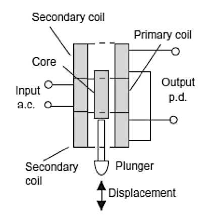
Figure: Figure: Normally Open contacts: The input contacts (IN1 etc) are not real contacts, they are part of the program.

Inductance Transducers

5 way 2 position Plunger Spring Valve

Figure 13. Linear Variable Differential Transformer (LVDT)

Inductive transducers are used for proximity sensing and also for motion position detection, motion control and process control applications. They are based on the Faraday’s law of induction in a coil, which specifies that the induced voltage, or electromotive force (EMF), is equal to the rate at which the magnetic flux through the circuit changes. There are different ways how this can be exploited for the purpose of displacement transducers, and most commonly, it is the change in mutual inductance. The presence of an induced emf in one circuit due entirely to a chance in another circuit is called mutual induction. The most widely used inductance transducer is Linear Variable Differential Transformer (LVDT). LVDTis a transformer with a primary coil and two secondary coils.
Figure 13 shows the arrangement, there being three coils symmetrically spaced along an insulated tube. The central coil is the primary coil and the other two are identical secondary coils which are connected in series in such a way that their outputs oppose each other. A magnetic core is moved through the central tube as a result of the displacement being monitored. When there is an alternating voltage input to the primary coil, alternating emfs are induced in the secondary coils. With the magnetic core in a central position, the amount of magnetic material in each of the secondary coils is the same and so the emfs induced in each coil are the same. Since they are so connected that their outputs oppose each other, the net result is zero output. However, when the core is displaced from the central position there is a greater amount of magnetic core in one coil than the other. The result is that a greater emf is induced in one coil than the other and then there is a net output from the two coils. The bigger the displacement the more of the core there is in one coil than the other, thus the difference between the two e.m.f.s increases, the greater the displacement of the core.

Typically, LVDTs have operating ranges from about ±2 mm to ±400 mm. Non-linearity errors are typically about ±0.25%. LVDTs are very widely used for monitoring displacements. A commercially available displacement sensor using a LVDT has the following in its specification:

Ranges ±0.125 mm to ±470 mm
Non-linearity error ±0.25% of full range
Temperature sensitivity ±0.01% of full range

Digital Sensors for Motion Measurement

Digital transducers are ideal devices for motion measurement. They produce digital output which can be interfaced to the computer. They are very attractive because of their properties:

Signal conditioning simplicity
Resilience to electro-magnetic interference

Figure 14. Optical incremental encoder

Optical Encoders
An encoder is a device that provides a digital output as a result of an angular or linear displacement. Position encoders can be grouped into two categories: incremental encoders, which detect changes in displacement from some datum position, and absolute encoders, which give the actual position. Figure 14 shows the basic form of an incremental encoder for the measurement of angular displacement of a shaft. It consists of a disc which rotates along with the shaft. In the form shown, the rotatable disc has a number of windows through which a beam of light can pass and be detected by a suitable light sensor. When the shaft rotates and disc rotates, a pulsed output is produced by the sensor with the number of pulses being proportional to the angle through which the disc rotates. The angular displacement of the disc, and hence the shaft rotating it, can thus be determined by the number of pulses produced in the angular displacement from some datum position. Typically the number of windows on the disc varies from 60 to over a thousand with multi-tracks having slightly offset slots in each track. With 60 slots occurring with 1 revolution then, since 1 revolution is a rotation of 360°, the minimum angular displacement, i.e. the resolution, that can be detected is 360/60=6°. The resolution thus typically varies from about 6° to 0.3° or better.

Figure 15. The rotating wheel of the absolute encoder. Note that though the normal form of binary code is shown in the figure, in practice a modified form of binary code called the Gray code is generally used. This code, unlike normal binary, has only one bit changing in moving from one number to the next. Thus we have the sequence 0000, 0001, 0011, 0010, 0011, 0111, 0101, 0100, 1100, 1101, 1111
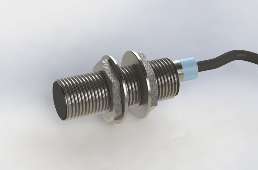
Inductivity Proximity Sensor

An Inductivity Proximity Sensor is basically a coil which has an alternating current applied to it to produce an alternating magnetic field which is sensed by another coil (Figure 24). When a metallic object is moved close to the coil it disturbs the magnetic field and so the magnetic field detected by the sensing coil. Such a sensor can be used to detect metallic objects up to about 8 mm away.
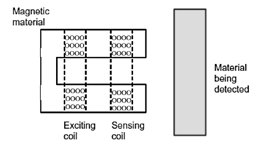Figure 24. Inductive Proximity Sensor

Eddy Current Transducer

When a conducting material is placed in a changing magnetic field, an electromotive force (EMF) is induced in it. This EMF causes localised currents to flow, which are known as eddy currents. Eddy currents can be induced in conductor but are most noticeable in solid conductors. For example when the magnetic core of transformer or rotating machine is subjected to a change in magnetisation, eddy currents are produced. Figure 25 shows principle behind the eddy current transducer.
Figure 25. Eddy Current Transducer principle

A nonferrous plate moves in a direction perpendicular to the lines of flux of a magnet. Eddy currents generated in the plate are proportional to the velocity of the plate. The eddy currents set up a magnetic field in a direction perpendicular to the lines of flux of a magnet. Eddy currents generated in the plate are proportional to the velocity of the plate. The eddy currents set up magnetic field in the direction, that opposes the magnetic field that creates them. The output voltage is proportional to the rate of change of eddy currents in the plate.

The eddy current sensor, shown in Figure 26, has two identical coils, one coil is used as a reference, and the second coil is used to sense the magnetic current in conductive object.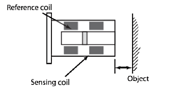
Figure 26. Sensing and Reference Coils in an Eddy Current Transducer

Eddy currents produce magnetic field, which opposes that of the sensing coil, resulting in a reduction of flux. When the plate is nearer to the coil, the eddy currents as well as the change in magnetic impedance are both larger. The coils form two arms of an impedance bridge. The bridge has a supply frequency usually of 1 MHz or higher. In the absence of a target object, the output of the impedance bridge is zero. As a target moves closer to the sensor, eddy current are generated in the conducting medium because of radio frequency (RF) magnetic flux from the active coil. Inductance of the active coil increases, causing the voltage output in bridge circuit.

Mechanical Switches

The basic part of a limit switch is an electrical switch which is switched on or off by means of a plunger(Figure 21(A)), the movement of this plunger being controlled by the actuator head of the limit switch which transfers the external force and movement to it. Depending on the object and movement being detected, the actuator head can take a number of forms. A common form is a roller rotating an arm to move a plunger inside the switch to activate the switch contacts and having a spring return (Figure 21(B)).
The way in which the plunger moves when making the switch contacts and when breaking them is determined by springs to enable the switch to be slow or fast acting when making or breaking contacts.

Figure 21. The basic form a limit switch: (A) the built-in switch with the contacts being switched by the movement of plunger, (B) a roller-actuated limit switch, rotation of the roller arm moving the plunger, and (C) a simple application of limit switches.

Mechanical Switches

There are many situations where a sensor is required to detect the presence of some object. The sensor used in such situations can be a mechanical switch, giving an on-off output when the switch contacts are opened or closed by the presence of an object. Switches are used for such applications as where a work piece closes the switch by pushing against it when it reaches the correct position on a work table, such a switch being referred to as a limit switch because they were first used to determine the limit of travel of a moving part and when an object has reached its end of travel. The switch might then be used to switch on a machine tool to carry out some operation on the work piece. Another example is a light being required to come on when a door is opened, as in a refrigerator. The action of opening the door can be made to close the contacts in a switch and trigger an electrical circuit to switch on the lamp. A similar application is to switch on the interior light in an automobile when a door is opened.
Another application is to sense the end-of-travel position for electric windows and switch off the motor moving the windows. Limit switches are widely used, being rugged, reliable and easily installed.

📷 The basic part of a limit switch is an electrical switch which is switched on or off by means of a plunger(Figure 21(A)), the movement of this plunger being controlled by the actuator head of the limit switch which transfers the external force and movement to it. Depending on the object and movement being detected, the actuator head can take a number of forms.

📷 A common form is a roller rotating an arm to move a plunger inside the switch to activate the switch contacts and having a spring return (Figure 21(B)).The way in which the plunger moves when making the switch contacts and when breaking them is determined by springs to enable the switch to be slow or fast acting when making or breaking contacts.

Figure 22 shows a form of a non-contact switch sensor, a reed switch. This consists of two overlapping, but not touching, strips of a spring magnetic material sealed in a glass or plastic envelope. When a magnet or current carrying coil is brought close to the switch, the strips become magnetised and attract each other. The contacts then close. Typically a magnet closes the contacts when it is about 1 mm from the switch.

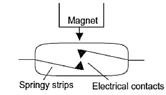Figure 22. Reed Switch

There are situations where detectors are required to be touch-sensitive, giving outputs when touched. One example of this used as a resistance element is a doped conductive elastomer. When it is touched, the pressure causes it to elastically indent and become compressed. This increases the doping density in that region and so results in a resistance change. Such sensors have been developed in the form of the doped elastomer in the form of cords and laid in a grid pattern with the resistances being monitored at the points of intersection to yield information about which ones have been touched and so give information about the size and shape of the object in contact with the grid. A sensor that has been used with robot hands to monitor the force exerted when the hand grips an object involves a plunger being moved by the force and interrupting the light beam from a LED and hence the output from a light sensor (Figure 23).

Figure 23. Touching causes the plunger to interrupt the light beam and so the signal detected by the light sensor

Capacity Proximity sensors

A proximity sensor that can be used with metallic and non-metallic objects is the capacitive proximity sensor. This is a non-contact sensor which has a probe which essentially consists of a pair of parallel capacitor plates between which a potential difference is applied to produce an electric field. This field is disturbed when it is moved close to an object. Thus the proximity of the object is detected by a change in capacitance. The sensor can also be used to detect a wide variety of non- metallic and metallic objects and typically operate over a range of 3 to 30 mm.

Optical Range Sensors

Range sensing techniques are of special importance in manufacturing automation applications. They have been successfully employed in some other areas such as: automatic guidance systems of vehicles, Robot Navigations, Collision avoidance and similar. They are mainly optical, so we will explain the basic ones here, but the same principles apply for non-optical methods as well. The basic principle on which most of these techniques are based is the triangulation principle, which applies trigonometric principles to determine the distance of an object from two previously known positions. Figure 30 illustrates the principle in a thickness-measuring application.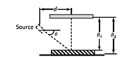

Figure 30. Triangulation principle to measure thickness (R₁-R₂)

The source, typically a laser, is focused on the surface of the object. A photodetector is used to determine the location of the spot. The distance, R₂, and angle, $ \Theta$, are known. Because the photodetector is located at a fixed distance in the work environment, the thickness of the part is calculated as $$ T = R_2 - R_1 = R_2 - d \; tan \; \Theta $$ Here $d$ is found from the position of the light spot on the workpiece.

If two triangulation sensors are positioned a certain distance apart and both devices can align to a spot on an object, as shown in Figure 31, then the two devices and the object form a triangle. The distance, $d$, and two angles, $ \Theta _1$ and $ \Theta _2$, are known. The third angle is found by subtracting two know angles from 180°.

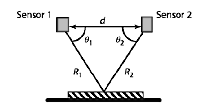Figure 31. Triangulation Principle with Two Sensors

The distance from each device to the object can then be found using the law of sines: $$ R _1 = \frac{d \; sin \; \Theta _2}{sin \; (180 - (\Theta _1 + \Theta _2))} $$ $$ R _2 = \frac{d \; sin \; \Theta _1}{sin \; (180 - (\Theta _1 + \Theta _2))} $$ Instrumental techniques using triangulation principles include following six methods:

1. Spot sensing method
2. Light strip sensing method
3. Camera motion method
4. Time of flight technique
5. Binocular vision technique
6. Optical ranging using position sensitive detectors

Beside these techniques, the distance can be also optically measured using laser interferometer, where the distance can be determined in the terms of wavelengths by examining the phase relation between a reference bean and laser beam reflected from a target object.

💡MINI QUIZ

Example 3: Logical AND Function (Contacts in Series)

Figure shows an AND function.

When Switches SW1 AND SW2 are closed IN1 AND IN2 contacts close energising the control relay RC1 turning ON the load.

It is important to note that closing only one switch will not turn on the load.

Figure: Logical AND with PLC software

Example 4: Logical OR Function (Contacts in Parallel)

Figure shows an OR function.

When Switches Sw1 OR Sw2 are closed IN1 OR IN2 contacts close energising the control relay RC1 turning ON the load.

It is important to note that closing only one switch is sufficient to turn on the load.

Figure: Logical OR with PLC software

Example 5: Combined Logical AND and OR Functions (Contacts in Parallel & Series)

Figure shows an example which uses combinations of normally open contacts, normally closed contacts, AND and OR functions.

Closing Sw1 or Sw2 will close contacts IN1 OR IN2 respectively and the control relay RC1 will be energised through the normally closed contacts IN3, turning ON the load

When Sw3 is closed IN3 contacts will open so the load will be turned OFF.

Figure: Combined Logical AND and OR with PLC software

Mechanical Switches

Figure 27 shows the Hall effect principle. Current is passed through leads 1 and 2 of the element. The output ends will produce zero voltage when there is no transverse magnetic field passing through element. When there is a magnetic flux passing through the element, a voltage $V$ appears between output leads. This voltage is proportional to the current and field strength. The output voltage is represented in terms of element thickness, the flux intensity of the field, the current through the element, and the Hall coefficient as: $$ V = H \frac{IB}{T} $$ Where:

$H$ = Hall coefficient, which can be defined as transverse electric potential gradient per unit magnetic field per unit current density. The units are Vm³/AWb.

$I$ = current through the Element (A)

$B$ = flux density (Wb/m²)

$T$ = thickness of the element (m)

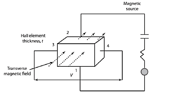Figure 27. Hall Effect Principle

Question #1 - Ultrasonic sensors use the following signal for measurement: Light Sound Electrical Voltage	Question #2 - Optical Range Sensors are mainly optical: False True

Hall Effect Transducer

Figure 27. Hall Effect Principle

The Hall effect results in the production of an electric field perpendicular to the directions of both the magnetic field and the current with a magnitude proportional to the product of magnetic field strength, the current, and various properties of conductor. An electron, with charge $e$, traveling in a magnetic field $\vec B$, with a velocity $\vec v$, experiences a Lorenz force $\vec F$, which is given by: $$ \vec F = e ( \vec v \times \vec B ) $$ An electric field, known as Hall’s field, counterbalances Lorenz’s force and is represented by an electric potential. The voltage produced may be used to produce field strength or current.
📷 Figure 27 shows the Hall effect principle. Current is passed through leads 1 and 2 of the element.The output ends will produce zero voltage when there is no transverse magnetic field passing through element. When there is a magnetic flux passing through the element, a voltage $V$ appears between output leads. This voltage is proportional to the current and field strength. The output voltage is represented in terms of element thickness, the flux intensity of the field, the current through the element, and the Hall coefficient as: $$ V = H \frac{IB}{T} $$ Where:

$H$ = Hall coefficient, which can be defined as transverse electric potential gradient per unit magnetic field per unit current density. The units are Vm³/AWb.

$I$ = current through the Element (A)

$B$ = flux density (Wb/m²)

$T$ = thickness of the element (m)

Figure 28 shows the principal application of the Halls effect for distance measurement. As the magnet moves back and forth at that fixed gap, the magnetic field induced by the element becomes negative as it approaches the north pole and positive, as it approaches the south pole.

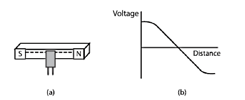Figure 28. Hall Effect Transducer (A) Principle (B) Input/Output Characteric Curve

Ultrasonic Distance Sensor

The ultrasonic transducer emits a pulse of ultrasonic wave and then receives echo from the object targeted. Ultrasonic waves have higher than audible frequency of 20kHz. The ultrasonic transduces consists of a transmitter, a receiver, and a processing unit. These transducers usually produce waves in the frequency range of 30 to 100 kHz. When ultrasonic beam reaches a surface, one portion of beam is absorbed by the medium, another reflected, and third portion is transmitted through the medium.

Figure 29. Ultrasonic Distance Sensor

Figure 29 presents principle of work of ultrasonic distance sensor. Transmitter sends ultrasonic wave, with speed $v$, to the object at the distance $d$, and with the incident angle $\Theta$. The time for the ultrasonic wave to travel from the transmitter to the object and back to receiver is $t$. Using the definition we can derive equation: $$ d = \frac{vt \; cos \; \Theta}{2} $$ Measuring $t$, we can derive the distance $d$. For longer distances angle $\Theta$ could be approximate to zero, simplifying the calculation. The accuracy of the ultrasonic transducer is high and often in the order of one percent of the range measured. The sensors are used in robotics applications, where robot manipulators need to avoid collisions and sense the distance of the object or obstruction in the vicinity of robot workspace.