-
Fluid pressure and flow and liquid level sensors
Many of the devices used to monitor fluid pressure in industrial processes involve the monitoring of the elastic deformation of diaphragms, bellows, and tubes. The following are some common examples of such sensors. The term absolute pressure is used for a pressure measured relative to a vacuum, differential pressure when the difference between two pressures is measured and gauge pressure for the pressure measured relative to some fixed pressure, usually the atmospheric pressure. -
Piezoelectric Sensor
- When certain crystals are stretched or compressed, charges appear on their surfaces. This effect is called piezoelectricity. Examples of such crystals are quartz, tourmaline, and zirconate-titanate.
A piezoelectric pressure gauge consists essentially of a diaphragm which presses against a piezoelectric crystal (Figure 4). Movement of the diaphragm causes the crystal to be compressed and so charges produced on its surface. The crystal can be considered to be a capacitor which becomes charged as a result of the diaphragm movement and so a potential difference appears across it. The amount of charge produced and hence the potential difference depends on the extent to which the crystal is compressed and hence is a measure of the displacement of the diaphragm and so the pressure difference between the two sides of the diaphragm. If the pressure keeps the diaphragm at a particular displacement, the resulting electrical charge is not maintained but leaks away. Thus the sensor is not suitable for static pressure measurements. Typically such a sensor can be used for pressures up to about 1000 MPa with a non-linearity error of about ±1.0% of the full range value.
A commercially available piezoelectric diaphragm pressure gauge has in its specification:- • Ranges 0 to 20 MPa, 0 to 200 MPa, 0 to 500 MPa, 0 to 1000 MPa,
• Non-linearity error ±0.5%,
• Sensitivity -0.1 pC/kPa,
• Temperature sensitivity ±0.5% of full scale for use +20°C to +100°C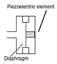 Figure 4. Basic form of a piezoelectric sensor
Bourdon Tube
- 📷 Bourdon tube instruments diagram larger
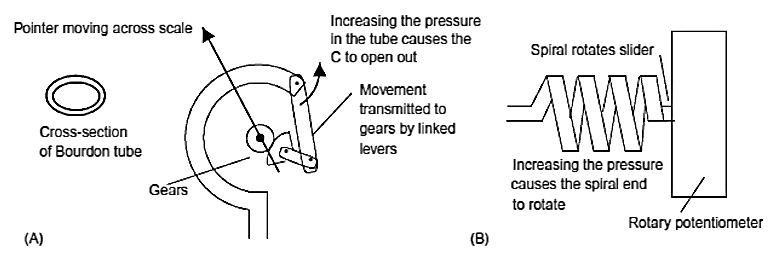 Figure 5. Bourdon tube instruments: (A) geared form, (B) potentiometer form
The Bourdon tube is an almost rectangular or elliptical cross-section tube made from materials such as stainless steel or phosphor bronze. With a C-shaped tube (Figure 5(A)), when the pressure inside the tube increases the closed end of the C opens out, thus the displacement of the closed end becomes a measure of the pressure. A C-shaped Bourdon tube can be used to rotate, via gearing, a shaft and cause a pointer to move across a scale.Such instruments are robust and typically used for pressures in the range 10 kPa to 100 MPa with an accuracy of about ±1% of full scale.
Another form of Bourdon instrument uses a helical-shaped tube (5(B)). When the pressure inside the tube increases, the closed end of the tube rotates and thus the rotation becomes a measure of the pressure. A helical-shaped Bourdon tube can be used to move the slider of a potentiometer and so give an electrical output related to the pressure. Helical tubes are more expensive but have greater sensitivity. Typically they are used for pressures up to about 50 MPa with an accuracy of about ±1% of full range.
Continues on next tab
Diaphragm Sensor
- The movement of the centre of a circular diaphragm as a result of a pressure difference between its two sides is the basis of a pressure gauge (Figure 1(A)). For the measurement of the absolute pressure, the opposite side of the diaphragm is a vacuum; for the measurement of pressure difference, the pressures are connected to each side of the diaphragm; for the gauge pressure, i.e. the pressure relative to the atmospheric pressure, the opposite side of the diaphragm is open to the atmosphere. The amount of movement with a plane diaphragm is fairly limited; greater movement can, however, be produced with a diaphragm with corrugations (Figure 1(B)).
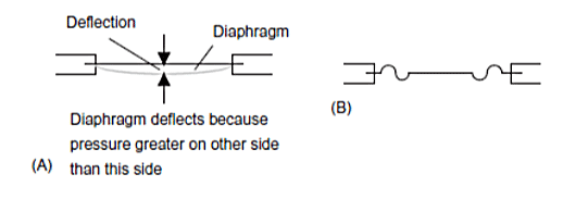 Figure 1. Diaphragm Pressure Sensors
The movement of the centre of a diaphragm can be monitored by some form of displacement sensor. Figure 2 shows the form that might be taken when strain gauges are used to monitor the displacement, the strain gauges being stuck to the diaphragm and changing resistance as a result of the diaphragm movement. Typically such sensors are used for pressures over the range 100 kPa to 100 MPa, with an accuracy up to about ±0.1%.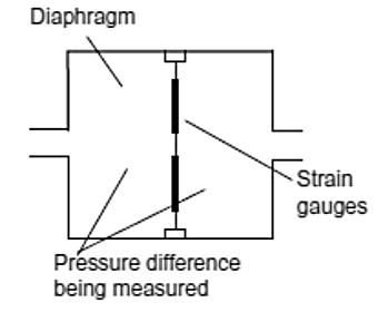 Figure 2. Diaphragm Pressure
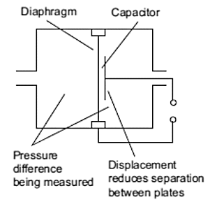 Figure 3. Diaphragm gauge using capacitance
Figure 3 shows the form that might be taken by a capacitance diaphragm pressure gauge. The diaphragm forms one plate of a capacitor, the other plate being fixed. Displacement of the diaphragm results in changes in capacitance. The range of such pressure gauges is about 1 kPa to 200 kPa with an accuracy of about ±0.1%.
Another form of diaphragm sensor uses a LVDT to monitor the displacement of the diaphragm. Such an arrangement is typically used for low pressure measures where high stability is required. The total error due to non-linearity, hysteresis, and repeatability can be of the order of ±0.5% of full scale.
(Cont.)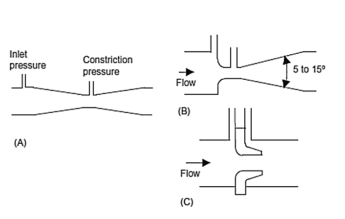 Figure 8.
(A) Venturi Tube,
(B) Venturi nozzle,
(C) Flow nozzle
The venturi tube (Figure 8 (A)) has a gradual tapering of the pipe from the full diameter to the constricted diameter. The presence of the venturi tube results in a pressure loss occurring in the system of about 10 to 15%, a comparatively low value. The pressure difference between the flow prior to the constriction and the constriction can be measured with a simple U-tube manometer or a differential diaphragm pressure cell. The instrument can be used with liquids containing particles, is simple in operation, capable of accuracy of about ±0.5%, has a longterm reliability, but is comparatively expensive and has a non-linear relationship between pressure and the volume rate of flow.
A cheaper form of venturi is provided by the nozzle flow meter (Figure 8). Two types of nozzle are used, the venturi nozzle and the flow nozzle. The venturi nozzle (Figure 8(B)) is effectively a venturi tube with an inlet which is considerably shortened. The flow nozzle (Figure 8(C)) is even shorter. Nozzles produce pressure losses of the order of 40 to 60%. Nozzles are cheaper than venturi tubes, give similar pressure differences, and have an accuracy of about ±0.5%. They have the same non- linear relationship between the pressure and the volume rate of flow.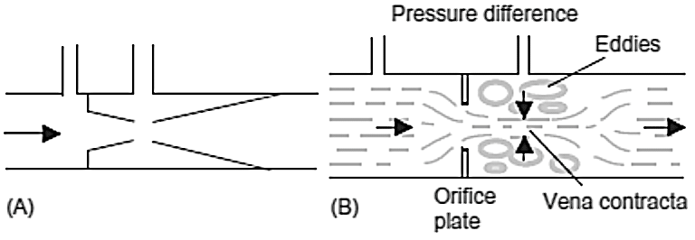 Figure 9. (A) Dall tube, (B) Orifice plate
- The Dall tube (Figure 9 (A)) is another variation of the venturi tube. It gives a higher differential pressure and a lower pressure drop. The Dall tube is only about two pipe diameters long and is often used where space does not permit the use of a venturi tube. The orifice plate (Figure 9 (B)) is simply a disc with a hole. The effect of introducing it is to constrict the flow to the orifice opening and the flow channel to an even narrower region downstream of the orifice. The narrowest section of the flow is not through the orifice but downstream of it and is referred to as the vena contracta. The pressure difference is measured between a point equal to the diameter of the tube upstream of the orifice and a point equal to half the diameter downstream. The orifice plate has the usual non-linear relationship between the pressure difference and the volume rate of flow. It is simple, reliable, produces a greater pressure difference than the venturi tube and is cheaper but less accurate, about ±1.5%. It also produces a greater pressure drop. Problems of silting and clogging can occur if particles are present in liquids.
Continues on next tab
Fluid Flow sensors
- Physics of Fluid Flow
The movement of a fluid through a pipe is obeys two principals of Mechanics of Fluids: Law of Continuity and Bernoulli’s Equation.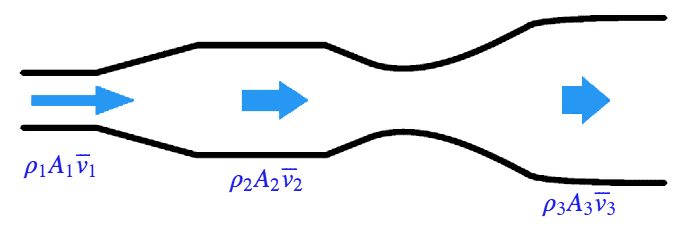 Figure 6. Flow stream of a fluid
Law of Continuity states that the product of average velocity ($v$), pipe cross-sectional area ($A$), and fluid density ($\rho$) for a given flow stream (Figure 6) must remain constant: $$ \rho _1 A _1 \overline{v_1} = \rho _2 A _2 \overline{v_2} = ..... = \rho _n A _n \overline{v_n} $$ This means that we may define product $\rho A v$ as an expression of mass flow rate, or $W$: $$ W = \rho A \overline{v} = const $$ Bernoulli’s equation is an expression of the Law of Energy Conservation for an inviscid (frictionless) fluid stream, named after Daniel Bernoulli. It states that the sum total energy at any point in a passive fluid stream (i.e. no pumps or other energy-imparting machines in the flow path, nor any energy-dissipating elements) must be constant (Figure 7):
y1ρg +$ \large \frac{v _1^2 \rho}{2}$ + P1 = y2ρg + $ \large \frac{v _2^2 \rho}{2}$ + P2
Where:
y = Height of fluid (from common reference point)
𝜌 = Mass density of fluid
g = Acceleration of gravity
v = Velocity of fluid
P = Pressure of fluid
Each of the three terms in Bernoulli’s equation is an expression of a different kind of energy, commonly referred to as head:
Elevation head y 𝜌 g
Velocity head $ \; \large \frac{v ^2 \rho}{2} $
Pressure Head P
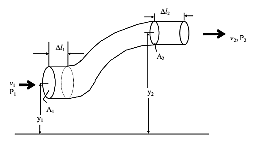 Figure 7. Bernoulli Equation Illustration
Differential Pressure Methods
- There are a number of forms of differential pressure devices based on the above equation and involving constant size constrictions, e.g. the venturi tube, nozzles, Dall tube and orifice plate. In addition there are other devices involving variable size constrictions, e.g. the rotameter. The following are discussions of the characteristics of the above devices.
(Cont.)- If the fluid going through the venturi tube is a liquid under relatively low pressure, we may vividly show the pressure at different points in the tube by means of piezometers, which are transparent tubes allowing us to view liquid column heights. The greater the height of liquid column in the piezometer, the greater the pressure at that point in the flowstream (Figure 12).
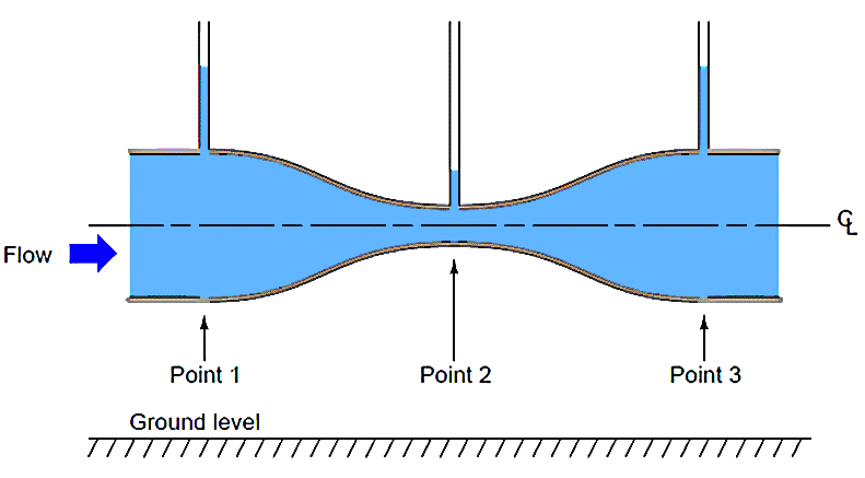 Figure 12. Venturi Tube
Solving the system equations derived from the Law of Continuity and the Bernoulli’s equation, we can find out that the velocity v2 if we know the pressures P1 and P2 is given by:
$$ \large v _2 =\sqrt{2} \frac{\large 1}{\sqrt{\large 1 - (\large \frac{A_2}{ A_1})^2 }} \sqrt{\large \frac{p_1 - p_2}{\rho}} $$
This shows us how to solve for fluid velocity at the venturi throat (v2) based on a difference of pressure measured between the mouth and the throat (P1 − P2). We are only one step away from a volumetric flow equation here, and that is to convert velocity (v) into flow rate (Q). Velocity is expressed in units of length per time (feet or meters per second or minute), while volumetric flow is expressed in units of volume per time (cubic feet or cubic meters per second or minute). Simply multiplying throat velocity (v2) by throat area (A2) will give us the result we seek:
Q = Av and: $$ \large Q =\sqrt{2} \;\; A_2 \frac{\large 1}{\sqrt{\large 1 - (\large \frac{A_2}{ A_1})^2 }} \sqrt{\large \frac{p_1 - p_2}{\rho}} $$ Please note how many constants we have in this equation. For any given venturi tube, the mouth and throat areas (A1 and A2) will be fixed. This means nearly half the variables found within this rather long equation are actually constant for any given Venturi tube, and therefore do not change with pressure, density, or flow rate. Knowing this, we may re-write the equation as a simple proportionality: $$Q = k \; \sqrt{\frac{P _2 - P_2}{\rho}} $$ Sometimes it is preferred the measurement of mass flow over the measurement of volumetric flow, but given simple relation between volume (V) and mass (m) for a sample of fluid with its mass density r $$ m = \rho V $$ We can easily find the mass flow rate (W) as: $$ W = \rho Q $$ And $$ W = k \sqrt{ \rho (P _1 - P _2)} $$
Question #1 - Fluid pressure sensors can be made with strain gauges:
Question #2 - Fluid flow sensors always use pressure measurement:
Differential Pressure Methods (Cont.)
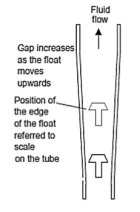 Figure 10. Rotameter
- The rotameter (Figure 10) is an example of a variable area flow meter; a constant pressure difference is maintained between the main flow and that at the constriction by changing the area of the constriction. The rotameter has a float in a tapered vertical tube with the fluid flow pushing the float upwards. The fluid has to flow through the constriction which is the gap between the float and the walls of the tube and so there is a pressure drop at that point. Since the gap between the float and the tube walls increases as the float moves upwards, the pressure drop decreases. The float moves up the tube until the fluid pressure is just sufficient to balance the weight of the float. The greater the flow rate the greater the pressure difference for a particular gap and so the higher up the tube the float moves. A scale alongside the tube can thus be calibrated to read directly the flow rate corresponding to a particular height of the float. The rotameter is cheap, reliable, has an accuracy of about ±1% and can be used to measure flow rates from about 30×10-6 m3/s to 1 m3/s.
The Pitot tube can be used to directly measure the velocity of flow of a fluid, rather than the volume rate of flow and consists essentially of just a small tube inserted into the fluid with an opening pointing directly upstream (Figure 11). The fluid impinging on the open end of the tube is brought to rest and the pressure difference measured between this point and the pressure in the fluid at full flow. The difference in pressure between where the fluid is in full flow and the point where it is stopped is due to the kinetic energy of the fluid being transformed to potential energy, this showing up as an increase in pressure. Because kinetic energy is mv2/2, the velocity is proportional to the square root of the pressure difference.
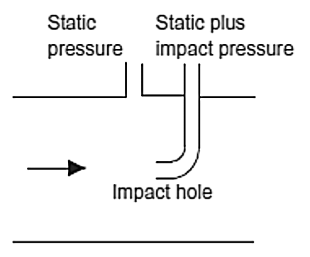 Figure 11. Pitot tube
The standard “textbook example” flow element used to create a pressure change by accelerating a fluid stream is the venturi tube: a pipe purposefully narrowed to create a region of low pressure. As shown previously, venturi tubes are not the only structure capable of producing a flow-dependent pressure drop. You should keep this in mind as we proceed to derive equations relating flow rate with pressure change: although the venturi tube is the canonical form, the exact same mathematical relationship applies to all flow elements generating a pressure drop by accelerating fluid, including orifice plates, flow nozzles, V-cones, segmental wedges, pipe elbows, pitot tubes, etc.
(Cont.)
This alternating series of vortices was studied by Vincenc Strouhal in the late nineteenth century and later by Theodore von Kármán in the early twentieth century. It was determined that the distance between successive vortices downstream of the stationary object is relatively constant, and directly proportional to the width of the object, for a wide range of Reynolds number values. If we view these vortices as crests of a continuous wave, the distance between vortices may be represented by the symbol customarily reserved for wavelength: the Greek letter “lambda” (λ), Figure 17.
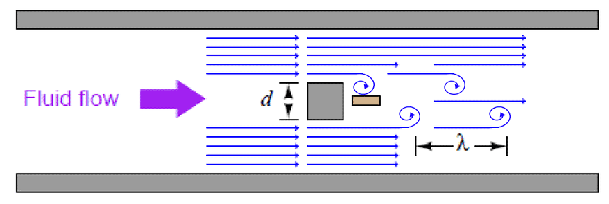 Figure 17. Vortex flowmeter principle
- The proportionality between object width (d) and vortex street wavelength (λ) is called the Strouhal number (S), approximately equal to 0.17:
𝜆 S = d
𝜆 ≈ $ \large \frac{d}{0.17} $
If a differential pressure sensor is installed immediately downstream of the stationary object in such an orientation that it detects the passing vortices as pressure variations, an alternating signal will be detected, Figure 18
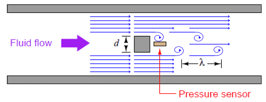 Figure 18. Vortex flowmeter with pressure sensor
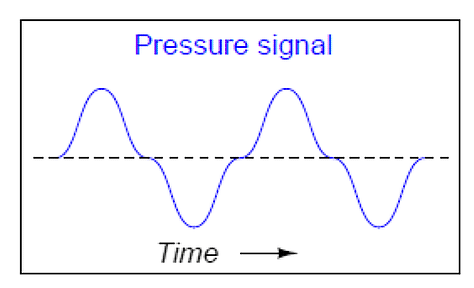 Figure 19. Variation of pressure in the Vertix Flowmeter, Figure 18
The frequency of this alternating pressure signal is directly proportional to fluid velocity past the object, since the wavelength is constant. This follows the classic frequency-velocity-wavelength formula common to all traveling waves (λf = v). Since we know the wavelength will be equal to the bluff body’s width divided by the Strouhal number (approximately 0.17), we may substitute this into the frequency-velocity-wavelength formula to solve for fluid velocity (v ) in terms of signal frequency (f ) and bluff body width (d ).
Turbine Meter
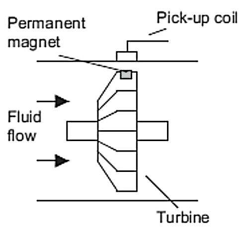 Figure 13. Basic principle of the turbine flowmeter
- The turbine flowmeter (Figure 13) consists of a multi-bladed rotor that is supported centrally in the pipe along which the flow occurs. The rotor rotates as a result of the fluid flow, the angular velocity being approximately proportional to the flow rate. The rate of revolution of the rotor can be determined by attaching a small permanent magnet to one of the blades and using a pick-up coil. An induced EMF pulse is produced in the coil every time the magnet passes it. The pulses are counted and so the number of revolutions of the rotor can be determined. The meter is expensive, with an accuracy of typically about ±0.1%. Another form uses helical screws which rotate as a result of the fluid flow.
Ultrasonic Flowmeters
- Ultrasonic flowmeters measure fluid velocity by passing high-frequency sound waves along the fluid flow path. Fluid motion influences the propagation of these sound waves, which may then be measured to infer fluid velocity. Two major sub-types of ultrasonic flowmeters exist: Doppler and transit-time. Both types of ultrasonic flowmeter work by transmitting a high-frequency sound wave into the fluid stream (the incident pulse) and analysing the received pulse.
Doppler flowmeters exploit the Doppler effect, which is the shifting of frequency resulting from waves emitted by or reflected by a moving object. A common realization of the Doppler effect is the perceived shift in frequency of a horn’s report from a moving vehicle: as the vehicle approaches the listener, the pitch of the horn seems higher than normal; when the vehicle passes the listener and begins to move away, the horn’s pitch appears to suddenly “shift down” to a lower frequency. In reality, the horn’s frequency never changes, but the velocity of the approaching vehicle relative to the stationary listener acts to “compress” the sonic vibrations in the air. When the vehicle moves away, the sound waves are “stretched” from the perspective of the listener.
The same effect takes place if a sound wave is aimed at a moving object, and the echo’s frequency is compared to the transmitted (incident) frequency. If the reflected wave returns from a bubble advancing toward the ultrasonic transducer, the reflected frequency will be greater than the incident frequency. If the flow reverses direction and the reflected wave returns from a bubble traveling away from the transducer, the reflected frequency will be less than the incident frequency.
This matches the phenomenon of a vehicle’s horn pitch seemingly increasing as the vehicle approaches a listener and seemingly decreasing as the vehicle moves away from a listener (Figure 14)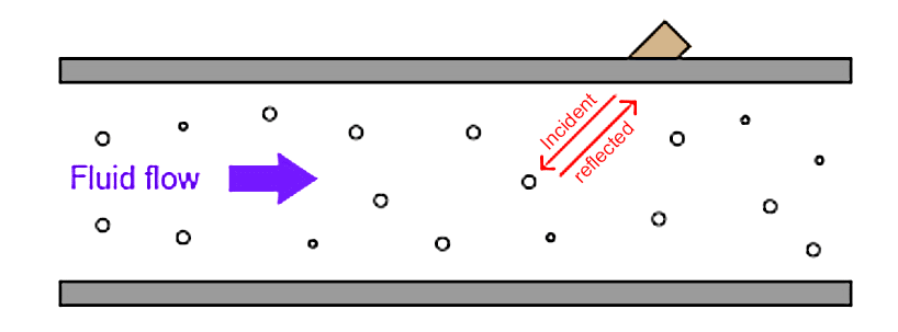 Figure 14. Ultrasonic flowmeter
Vortex Flowmeters
- When a fluid moves past a stationary object (a “bluff body”), there is a tendency for the fluid to form vortices on either side of the object. Each vortex will form, then detach from the object and continue to move with the flowing gas or liquid, one side at a time in alternating fashion. This phenomenon is known as vortex shedding, and the pattern of moving vortices carried downstream of the stationary object is known as a vortex street.
It is commonplace to see the effects of vortex shedding on a windy day by observing the motion of flagpoles, light poles, and tall smokestacks. Each of these objects has a tendency to oscillate perpendicular to the direction of the wind, owing to the pressure variations caused by the vortices as they alternately form and break away from the object, Figure 16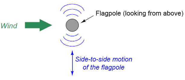 Figure 16. Wind passing flagpole
Liquid Level Sensors
- Methods used to measure the level of liquid in a vessel include those based on:
1. Floats whose position is directly related to the liquid level.2. Archimedes’ principle and a measurement of the upthrust acting on an object partially immersed in the liquid; the term displacer is used.3. A measurement of the pressure at some point in the liquid, the pressure due to a column of liquid of height h being hρg, where ρ is the liquid density, and g the acceleration due to gravity.4. A measurement of the weight of the vessel containing the liquid plus liquid. The weight of the liquid is Ahρg, where A is the cross-sectional area of the vessel, h the height of liquid, ρ its density, and g the acceleration due to gravity and thus changes in the height of liquid give weight changes.5. A change in electrical conductivity when the liquid rises between two probes.6. A change in capacitance as the liquid rises up between the plates of a capacitor.7. Ultrasonic and nuclear radiation methods.
The following gives examples of the above methods used for liquid level measurements.Floats
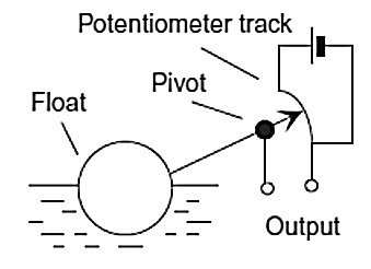 Figure 22. Potentiometar float gauge
- Figure 22 shows a simple float system. The float is at one end of a pivoted rod with the other end connected to the slider of a potentiometer. Changes in level cause the float to move and hence move the slider over the potentiometer resistance track and so give a potential difference output related to the liquid level. A problem with floats is that there is the problem of fluids and deposits coating the floats and changing the level at which they float.
Displacer Gauge
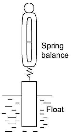 Figure 23. Displacer Gauge
- When an object is partially or wholly immersed in a fluid it experiences an upthrust force equal to the weight of fluid displaced by the object. This is known as Archimedes’ principle. Thus a change in the amount of an object below the surface of a liquid will result in a change in the upthrust. The resultant force acting on such an object is then its weight minus the upthrust and thus depends on the depth to which the object is immersed. For a vertical cylinder of cross-sectional area A in a liquid of density ρ, if a height h of the cylinder is below the surface then the upthrust is hAρg, where g is the acceleration due to gravity, and so the apparent weight of the cylinder is (mg - hAπg), where m is the mass of the cylinder. Such displacer gauges need calibrating for liquid level determinations for particular liquids since the upthrust depends on the liquid density. Figure 23 shows a simple version of a displacer gauge. A problem with displacers is that there is the problem of fluids coating the floats and apparently changing the buoyancy.
Differential Pressure
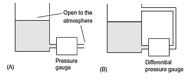 Figure 24. Pressure level gauges
The pressure due to a height h of liquid above some level is hρg, where ρ is the liquid density and g the acceleration due to gravity. With a tank of liquid open to the atmosphere, the pressure difference can be measured between a point near the base of the tank and the atmosphere. The result is then proportional to the height of liquid above the pressure measurement point (Figure 24(A)). With a closed tank, the pressure difference has to be measured between a point near the bottom of the tank and in the gases above the liquid surface (Figure 24(B)). The pressure gauges used for such measurements tend to be diaphragm instruments.
Magnetic Flowmeters
- When an electrical conductor moves perpendicular to a magnetic field, a voltage is induced in that conductor perpendicular to both the magnetic flux lines and the direction of motion. This phenomenon is known as electromagnetic induction, and it is the basic principle upon which all electro-mechanical generators operate.
In a generator mechanism, the conductor in question is typically a coil (or set of coils) made of copper wire. However, there is no reason the conductor must be made of copper wire. Any electrically conductive substance in motion is sufficient to electromagnetically induce a voltage, even if that substance is a liquid. Therefore, electromagnetic induction is a technique applicable to the measurement of liquid flow rates.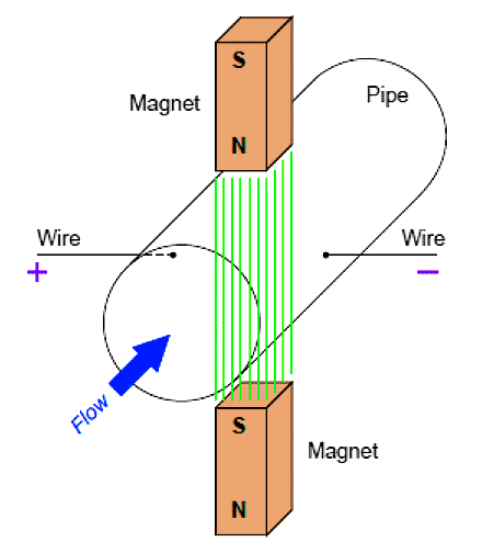 Figure 20. Magnetic Flowmeter
Consider water flowing through a pipe, with a magnetic field passing perpendicularly through the pipe, Figure 20.
Voltage induced by the linear motion of a conductor through magnetic field is called motional EMF, and it is proportional to the velocity of the conductor.
The direction of liquid flow cuts perpendicularly through the lines of magnetic flux, generating a voltage along an axis perpendicular to both. Metal electrodes opposite each other in the pipe wall intercept this voltage, making it readable to an electronic circuit.Optical Flowmeters
- A relatively recent development in industrial flow measurement is the use of light to measure the velocity of a fluid through a pipe. One such technology referred to as Laser-Two-Focus (L2F) uses two laser beams to detect the passage of any light-scattering particles carried along by the moving fluid, Figure 21.
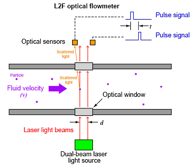 Figure 21. Optical flowmeter principle
$ \large v = \frac{d}{t} $Where,
v = Velocity of particle
d = Distance separating laser beams
t = Time difference between sensor pulses
As a particle passes through each laser beam, it redirects the light away from its normal straightline path in such a way that an optical sensor (one per beam) detects up the scattered light and generates a pulse signal. As that same particle passes through the second beam, the scattered light excites a second optical sensor to generate a corresponding pulse signal. The time delay between two successive pulses is inversely proportional to the velocity of that particle. This technique is analogous to that used by law-enforcement officers to measure the speed of a vehicle on a highway when viewed from an aircraft: measure how much time elapses as the vehicle passes between two marks on the road spaced a known distance from each other.
L2F flowmeters of course rely on the continual presence of light-scattering particles within the fluid. These particles could be either liquid droplets or solids within a gas stream, or they could be solid particles or bubbles in a liquid stream.Ultrasonic Level Gauge
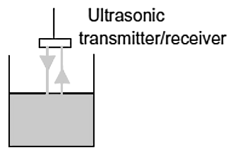 Figure 27. Ultrasonic gauge
- In one version of an ultrasonic level indicator, an ultrasonic transmitter/receiver is placed above the surface of the liquid (Figure 27). Ultrasonic pulses are produced, travel down to the liquid surface and are then reflected back to the receiver. The time taken from emission to reception of the pulses can be used as a measure of the position of the liquid surface. Because the receiver/transmitter can be mounted outside the liquid, it is particularly useful for corrosive liquids. Errors are produced by temperature changes since they affect the speed of the sound wave. Such errors are typically about 0.18% per °C.
Nucleonic Level Indicators
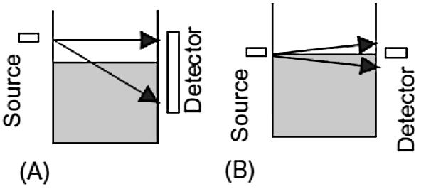 Figure 28. Radionic Gauges
- One form of level indicator uses gamma radiation from a radioactive source, generally cobalt-60, caesium-137, or radium-226. A detector is placed on one side of the container and the source on the other. Theintensity of the radiation depends on the amount of liquid between the source and detector and can be used to determine the level of the liquid.
Figure 28 shows two possible arrangements. With a compact source and extended detector, level changes over the length of the detector can be determined. A compact source and a compact detector can be used where small changes in a small range of level are to be detected. Such methods can be used for liquids, slurries, and solids, and, since no elements of the system are in the liquid, for corrosive and high temperature liquids.
Question #1 - Liquid level sensors can be made with strain gauges:
Question #2 - Continuity law is main principle on which liquid level measurement is based:
Load Cell
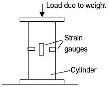 Figure 25. Load Cell
- The weight of a tank of liquid can be used as a measure of the height of liquid in the tank. Load cells are commonly used for such weight measurements. One form of load cell consists of a strain-gauged cylinder (Figure 25) which is included in the supports for the tank of liquid. When the level of the liquid changes, the weight changes and so the load on the load cell changes and the resistances of the strain gauges change. The resistance changes of the strain gauges are thus a measure of the level of the liquid. Since the load cells are completely isolated from the liquid, the method is useful for corrosive liquids.
Electrical Conductivity Level Indicator
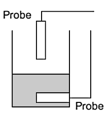 Figure 26.
- Conductivity methods can be used to indicate when the level of a high electrical conductivity liquid reaches a critical level. One form has two probes, one probe mounted in the liquid and the other either horizontally at the required level or vertically with its lower end at the critical level (Figure 26).
When the liquid is short of the required level, the resistance between the two probes is high since part of the electrical path between the two probes is air. However, when the liquid level reaches the critical level, there is a path entirely through the liquid and so the conductivity drops. Foaming, splashing, and turbulence can affect the results. - When certain crystals are stretched or compressed, charges appear on their surfaces. This effect is called piezoelectricity. Examples of such crystals are quartz, tourmaline, and zirconate-titanate.