-

Temperature Sensors
The expansion or contraction of solids, liquids, or gases, the change in electrical resistance of conductors and semiconductors, thermoelectric emfs, the change in the current across the junction of semiconductor diodes and transistors, or the energy and spectrum emitted by a body are all examples of properties that change when the temperature changes and can be used as basis of temperature sensors. In this module we will cover six most typical sorts of temperature sensors:
- Bimetal temperature sensors
- Liquid in glass temperature sensors
- Resistance Temperature Detectors (RTDs)
- Thermistors
- Thermocouples
- Non-contact temperature sensors
-
Liquid in Glass Temperature Sensors
- The liquid in glass thermometer involves a liquid expanding up a capillary tube. The height to which the liquid expands is a measure of the temperature. With mercury as the liquid, the range possible is -35°C to +600°C, with alcohol -80°C to +70°C, with pentane -200°C to +30°C. Such thermometers are direct reading, fragile, capable of reasonable accuracy under standardised conditions, fairly slow reacting to temperature changes, and cheap.
Resistance Temperature Detectors (RTDs)
- One of the simplest classes of temperature sensor is one where temperature effects a change in electrical resistance. With this type of primary sensing element, a simple ohmmeter is able to function as a thermometer, interpreting the resistance as a temperature measurement, Figure 3
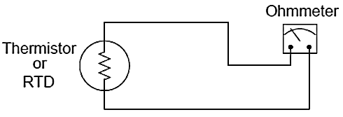 Figure 3. RTD (or Thermistor) measurement
A Resistance Temperature Detector (RTD) is a special temperature-sensing element made of fine metalwire, the electrical resistance of which changes with temperature as approximated by the following formula:RT = Rref [ 1 + $ \alpha $(T - Tref ) ]Where
RT = Resistance of RTD at given temperature $T (\Omega)$
Rref = Resistance of RTD at the reference Temperature Tref
$\alpha$ = Temperature coefficient of resistance (1/K)
RTDs are simple resistive elements in the form of coils of metal wire, e.g. platinum, nickel, or copper alloys. Platinum detectors have high linearity , Figure 4 (A) , good repeatability, high long-term stability, can give an accuracy of ±0.5% or better, a range of about -200°C to +850°C, can be used in a wide range of environments without deterioration, but are more expensive than the other metals. They are, however, very widely used. Nickel and copper alloys are cheaper but have less stability, are more prone to interaction with the environment, and cannot be used over such large temperature ranges.
A commercially available platinum resistance thermometer includes the following in its specification:
Range -200°C to +800°C
Accuracy ±0.01°C
Sensitivity 0.4 Ω/°C for 100 Ω
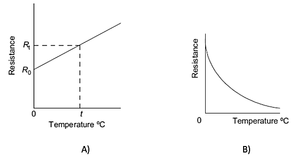 Figure 4. Resistance Variation with Temperature change for A) RTDs, B) Thermistors
Bimetal Temperature Sensors
- Solids tend to expand when heated. The amount that a solid sample will expand with increased temperature depends on the size of the sample, the material it is made of, and the amount of temperature rise. The following formula relates linear expansion to temperature change:
l = l0 (1 + 𝛼∆ T )Where:
𝑙 = Length of material after heating (m)
𝑙0 = Original length of material (m)
𝛼 = Coefficient of linear expansion (1/K)
∆𝑇 = Temperature change (K or °C)
Here are some typical values of α for common metals:
• Aluminium = 25 × 10−6 per °C
• Copper = 16.6 × 10⁻⁶ per °C
• Iron=12×10−6 per°C
• Tin = 20 × 10−6 per °C
• Titanium = 8.5 × 10⁻⁶ per °C
As you can see, the values for α are quite small. This means the amount of expansion (or contraction) for modest temperature changes are almost too small to see unless the sample size (l0) is huge. We can readily see the effects of thermal expansion in structures such as bridges, where expansion joints must be incorporated into the design to prevent serious problems due to changes in ambient temperature. However, for a sample the size of your hand the change in length from a cold day to a warm day will be microscopic.
One way to amplify the motion resulting from thermal expansion is to bond two strips of dissimilar metals together, such as copper and iron. If we were to take two equally-sized strips of copper and iron, lay them side-by-side, and then heat both of them to a higher temperature, we would see the copper strip lengthen slightly more than the iron strip (Figure 1)
 Figure 1. Expansions of two separate different metal strips under same temperature
If we bond these two strips of metal together, this differential growth will result in a bending motion greatly exceeding the linear expansion. This device is called a bimetal strip (Figure 2)
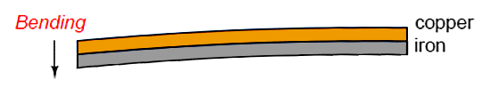 Figure 2. Bending of bonded bimetal strip under temperature
This bending motion is significant enough to drive a pointer mechanism, activate an electromechanical switch, or perform any number of other mechanical tasks, making this a very simple and useful primary sensing element for temperature. Older home thermostats often used this principle to both indicate room temperature and to actuate electrical switches for controlling room temperature. Electric hot water heater units still use this type of device (usually in the form of a convex bi-metal disk) to sense over-temperature conditions and automatically shut off power to the heater if the water temperature exceeds a pre-set limit.
Bimetallic strip devices are robust, relatively cheap, have an accuracy of the order of ±1%, and are fairly slow reacting to changes in temperature.Question #1 - Why do we need to use bimetal temperature sensors instead of single:
Question #2 - Which sensors show greatest linearity:
-
(Cont.)- Clearly, wire resistance is more problematic for low-resistance RTDs than for high-resistance thermistors. In the RTD circuit, wire resistance constitutes 1.96% of the total circuit resistance. In the thermistor circuit, the same 2 ohms of wire resistance constitutes only 0.004% of the total circuit resistance. The thermistor’s huge reference resistance value “swamps” the wire resistance to the point that the latter becomes insignificant by comparison.
In HVAC (Heating, Ventilation, and Air Conditioning) systems, where the temperature measurement range is relatively narrow, the nonlinearity of thermistors is not a serious concern and their relative immunity to wire resistance error is a definite advantage over RTDs. In industrial temperature measurement applications where the temperature ranges are usually much wider, the nonlinearity of thermistors becomes a significant problem, so we must find a way to use low-resistance RTDs and deal with the (lesser) problem of wire resistance.Four-wire RTD circuits
- A very old electrical measurement technique known as the Kelvin or four-wire method is a practical solution to the problem of wire resistance. Commonly employed to make precise resistance measurements for scientific experiments in laboratory conditions, the four-wire technique uses four wires to connect the resistance under test (in this case, the RTD) to the measuring instrument, which consists of a voltmeter and a precision current source. Two wires carry “excitation” current to the RTD from the current source while the other two wires merely “sense” voltage drop across the RTD resistor element and carry that voltage signal to the voltmeter. RTD resistance is calculated using Ohm’s Law: taking the measured voltage displayed by the voltmeter and dividing that figure by the regulated current value of the current source.
📷 A simple 4-wire RTD circuit is shown in Figure 7 for illustration.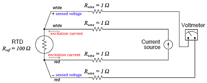 Figure 7. RTD connected to a Voltmeter in four-wire configuration
Wire resistances are completely inconsequential in this circuit. The two “excitation” wires carrying current to the RTD will drop some voltage along their length, but this voltage drop is only “seen” by the current source and not the voltmeter. The two “sense” wires connecting the voltmeter to the RTD also possess resistance, but they drop negligible voltage because the voltmeter draws so little current through them. Thus, the resistances of the current-carrying wires are of no effect because the voltmeter never senses their voltage drops, and the resistances of the voltmeter’s sensing wires are of no effect because they carry practically zero current.
Note how wire colours (white and red) indicate which wires are common pairs at the RTD. The RTD is polarity-insensitive because it is nothing more than a resistor, which is why it doesn’t matter which colour is positive and which colour is negative.
The only disadvantage of the four-wire method is the sheer number of wires necessary. Four wires per RTD can add up to a sizeable wire count when many different RTDs are installed in a process area.
Thermistors
- Thermistors are semiconductor temperature sensors made from mixtures of metal oxides, such as those of chromium, cobalt, iron, manganese, and nickel. The resistance of thermistors decreases in a very non-linear manner with an increase in temperature, Figure 4 (B) illustrating this. The change in resistance per degree change in temperature is considerably larger than that which occurs with metals. For example, a thermistor might have a resistance of 29 kΩ at -20°C, 9.8 kΩ at 0°C, 3.75 kΩ at 20°C, 1.6 kΩ at 40°C, 0.75 kΩ at 60°C. The material is formed into various forms of element, such as beads, discs, and rods (Figure 5). Thermistors are rugged and can be very small, so enabling temperatures to be monitored at virtually a point.
Because of their small size they have small thermal capacity and so respond very rapidly to changes in temperature. The temperature range over which they can be used will depend on the thermistor concerned, ranges within about -100°C to +300°C being possible. They give very large changes in resistance per degree change in temperature and so are capable, over a small range, of being calibrated to give an accuracy of the order of 0.1°C or better. However, their characteristics tend to drift with time. Their main disadvantage is their non-linearity. Thermistors are commonly used to monitor the coolant temperatures and the outside and internal air temperatures in automobiles.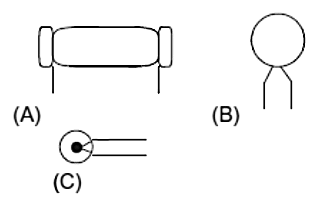 Figure 5. Thermistors: (A) rod, (B) disc, (C) bead shape
The following is part of the specification for a bead thermistor temperature sensor:
Accuracy ±5%
Maximum power 250 mW
Dissipation factor 7 mW/°C
Response time 1.2 s
Thermal time constant 11 s
Temperature range -40°C to +125°C
Practical issues with RTDs and Thermistor applications - Two wire RTD circuits
📷 The schematic diagrams in Figure 6 show the relative effects of 2 Ohms total wire resistance on a thermistor circuit (A) and on an RTD circuit(B)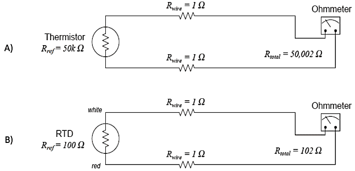 Figure 6. Thermistor (A) and RTD (B) connected to an Ohmmeter in two- wire configuration
As you can see, wire resistance adds to the sensing element’s resistance to create a larger total circuit resistance which will be interpreted by the receiving instrument (ohmmeter) as a falsely high temperature reading, assuming a positive temperature coefficient of resistance for the sensing element.
Two wire RTD circuits
The schematic diagrams in Figure 6 show the relative effects of 2 Ohms total wire resistance on a thermistor circuit (A) and on an RTD circuit(B)
Figure 6. Thermistor (A) and RTD (B) connected to an Ohmmeter in two- wire configuration
As you can see, wire resistance adds to the sensing element’s resistance to create a larger total circuit resistance which will be interpreted by the receiving instrument (ohmmeter) as a falsely high temperature reading, assuming a positive temperature coefficient of resistance for the sensing element.
Clearly, wire resistance is more problematic for low-resistance RTDs than for high-resistance thermistors. In the RTD circuit, wire resistance constitutes 1.96% of the total circuit resistance. In the thermistor circuit, the same 2 ohms of wire resistance constitutes only 0.004% of the total circuit resistance. The thermistor’s huge reference resistance value “swamps” the wire resistance to the point that the latter becomes insignificant by comparison.
In HVAC (Heating, Ventilation, and Air Conditioning) systems, where the temperature measurement range is relatively narrow, the nonlinearity of thermistors is not a serious concern and their relative immunity to wire resistance error is a definite advantage over RTDs. In industrial temperature measurement applications where the temperature ranges are usually much wider, the nonlinearity of thermistors becomes a significant problem, so we must find a way to use low-resistance RTDs and deal with the (lesser) problem of wire resistance.
Figure 7. RTD connected to a Voltmeter in four-wire configuration
Wire resistances are completely inconsequential in this circuit. The two “excitation” wires carrying current to the RTD will drop some voltage along their length, but this voltage drop is only “seen” by the current source and not the voltmeter. The two “sense” wires connecting the voltmeter to the RTD also possess resistance, but they drop negligible voltage because the voltmeter draws so little current through them. Thus, the resistances of the current-carrying wires are of no effect because the voltmeter never senses their voltage drops, and the resistances of the voltmeter’s sensing wires are of no effect because they carry practically zero current.
Note how wire colours (white and red) indicate which wires are common pairs at the RTD. The RTD is polarity-insensitive because it is nothing more than a resistor, which is why it doesn’t matter which colour is positive and which colour is negative.
The only disadvantage of the four-wire method is the sheer number of wires necessary. Four wires per RTD can add up to a sizeable wire count when many different RTDs are installed in a process area.
Figure: Output Module
- Clearly, wire resistance is more problematic for low-resistance RTDs than for high-resistance thermistors. In the RTD circuit, wire resistance constitutes 1.96% of the total circuit resistance. In the thermistor circuit, the same 2 ohms of wire resistance constitutes only 0.004% of the total circuit resistance. The thermistor’s huge reference resistance value “swamps” the wire resistance to the point that the latter becomes insignificant by comparison.
-
Thermocouples
- RTDs are completely passive sensing elements, requiring the application of an externally-sourced electric current in order to function as temperature sensors. Thermocouples, however, generate their own electric potential. In some ways, this makes thermocouple systems simpler because the device receiving the thermocouple’s signal does not have to supply electric power to the thermocouple.
It also makes thermocouple systems potentially safer than RTDs in applications where explosive compounds may exist in the atmosphere, because the power levels generated by a thermocouple tend to be less than the power levels dissipated by an RTD. The self-powering nature of thermocouples also means they do not suffer from the same “self-heating” effect as RTDs.
In other ways, however, thermocouple circuits are more complex and troublesome than RTD circuits because the generation of voltage actually occurs in two different locations within the circuit, not simply at the sensing point. This means the receiving circuit must “compensate” for temperature in another location in order to accurately measure temperature in the desired location.
Though typically not as accurate as RTDs, thermocouples are more rugged, have greater temperature measurement spans, and are easier to manufacture in different physical forms.
When two dissimilar metal wires are joined together at one end, a voltage is produced at the other end that is approximately proportional to temperature. That is to say, the junction of two different metals behaves like a temperature-sensitive battery. This form of electrical temperature sensor is called a thermocouple, Figure 9.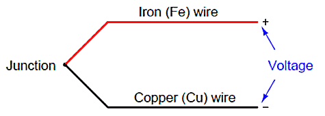 Figure 9. Thermocouple
This phenomenon provides us with a simple way to electrically infer temperature: simply measure the voltage produced by the junction, and you can tell the temperature of that junction. And it would be that simple, if it were not for an unavoidable consequence of electric circuits: when we connect any kind of electrical instrument to the thermocouple wires, we inevitably produce another junction of dissimilar metals. Figure 10 shows this fact, where the iron-copper junction J1 is necessarily complemented by a second iron-copper junction J2 of opposing polarity: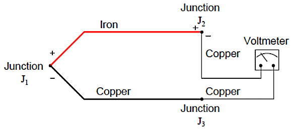 Figure 10. Thermocouple connected to a Voltmeter
Junction J1 is a junction of iron and copper – two dissimilar metals – which will generate a voltage related to temperature. Note that junction J2, which is necessary for the simple fact that we must somehow connect our copper-wired voltmeter to the iron wire, is also a dissimilar-metal junction which will also generate a voltage related to temperature. Further note how the polarity of junction J2 stands opposed to the polarity of junction J1 (iron = positive; copper = negative). A third junction (J3) also exists between wires, but it is of no consequence because it is a junction of two identical metals which does not generate a temperature-dependent voltage at all.
The presence of this second voltage-generating junction (J2) helps explain why the voltmeter registers 0 volts when the entire system is at room temperature: any voltage generated by the iron- copper junctions will be equal in magnitude and opposite in polarity, resulting in a net (series-total) voltage of zero. Only when the two junctions J1 and J2 are at different temperatures will the voltmeter register any voltage at all.
We may express this relationship mathematically as follows:
Vmeter = Vj1 - Vj2With the measurement (J1) and reference (J2) junction voltages opposed to each other, the voltmeter only “sees” the difference between these two voltages.
Thus, thermocouple systems are fundamentally differential temperature sensors. That is, they provide an electrical output proportional to the difference in temperature between two different points. For this reason, the wire junction we use to measure the temperature of interest is called the measurement junction while the other junction (which we cannot eliminate from the circuit) is called the reference junction (or the cold junction, because it is typically at a cooler temperature than the process measurement junction).
📷 Figure 11 (shown here) shows how the EMF varies with temperature for a number of commonly used pairs of metals.
Figure 18(A) illustrates this. Figure 18(B) shows a transmission form of instrument using Moiré fringes and Figure 18(C) a reflection form.
With both, a long grating is fixed to the object being displaced. With the transmission form, light passes through the long grating and then a smaller fixed grating, the transmitted light being detected by a photocell. With the reflection form, light is reflected from the long grating through a smaller fixed grating and onto a photocell. Coarse grating instruments might have 10 to 40 lines per millimetre, fine gratings as many as 400 per millimetre. Movement of the long grating relative to the fixed short grating results in fringes moving across the view of the photocell and thus the output of the cell is a sequence of pulses which can be counted. The displacement is thus proportional to the number of pulses counted. Displacements as small as 1 μm can be detected by this means. Such methods have high reliability and are often used for the control of machine tools.

Figure 18 (A) Moiré fringes, (B) transmission, and(C) reflection forms of instrument.Optical Proximity Sensors
- There are a variety of optical sensors that can be used to determine whether an object is present or not. Photoelectric switch devices can either operate as transmissive types where the object being detected breaks a beam of light, usually infrared radiation, and stops it reaching the detector (Figure 19(A)) or reflective types where the object being detected reflects a beam of light onto the detector (Figure 19(B)).
In both types the radiation emitter is generally a light-emitting diode (LED). The LED is a basic pn junction diode which emits light when suitable voltage is applied to it. The LED emits radiation which is reflected by the object. The reflected radiation is then detected by a phototransistor. In the absence of the object there is no detected reflected radiation; when the object is in the proximity, there is. The radiation detector might be a photodiode or a phototransistor, often a pair of transistors, known as a Darlington pair; using the pair increases the sensitivity.
Depending on the circuit used, the output can be made to switch to either high or low when light strikes the transistor. Such sensors are supplied as packages for sensing the presence of objects at close range, typically at less than about 5 mm.
Figure 19(C) shows a U-shaped form where the object breaks the light beam and so changes the response from a photodetector.
Another form of optical sensor is the pyroelectric sensor. Such sensors give a voltage signal when the infrared radiation falling on them changes, no signal being given for constant radiation levels. Lithium tantalate is a widely used pyroelectric material.
Figure 19. Photoelectric proximity sensors
Example 1: Normally Open Contacts
- Figure shows a practical example which uses normally open contacts in the ladder diagram
- When the switch is closed, $+24V$ is connected to IN1 of the PLC. This closes the contacts IN1 of the ladder diagram to energise control relay RC1 and hence turn load ON.
- If the switch is opened again, the contacts IN1 will spring open de-energising relay RC1 turning load OFF.
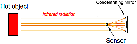
Figure: Normally Open contacts: The input contacts (IN1 etc) are not real contacts, they are part of the program.
 Figure 11. Generated potential (EMF) for various types of thermocouples
Type Positive wire characteristic Negative wire characteristic Plug Temp. range °C Sensitivity mV/ °C T Copper (blue)yellow coloured Constantan (red)silver coloured Blue -180 to 370 43 J Iron (white)magnetic, rusty Constantan (red)non-magnetic Black -180 to 760 53 E Chromel (violet)shiny finish Constantan (red)dull finish Violet 0 to 980 63 K Chromel (yellow)non-magnetic Alumel (red)magnetic Yellow -180 to 1260 41 R Pt87%-Rh13% (black) Platinum (red) Green 0 to1750 8
Table 1. Types of Thermocouples and their characteristics
Figure 11 shows how the EMF varies with temperature for a number of commonly used pairs of metals. Standard tables giving the EMFs at different temperatures are available for the metals usually used for thermocouples. Commonly used thermocouples are listed in Table 1, with the temperature ranges over which they are generally used and typical sensitivities. These commonly used thermocouples are given reference letters. The base-metal thermocouples, E, J, K, and T, are relatively cheap but deteriorate with age. They have accuracies which are typically about ±1 to 3%. Noble-metal thermocouples, e.g. R, are more expensive but are more stable with longer life. They have accuracies of the order of ±1% or better. Thermocouples are generally mounted in a sheath to give them mechanical and chemical protection. The response time of an unsheathed thermocouple is very fast. With a sheath this may be increased to as much as a few seconds if a large sheath is used.
Three-wire RTD circuits
📷 A compromise between two-wire and four-wire RTD connections is the three-wire connection is shown in Figure 8: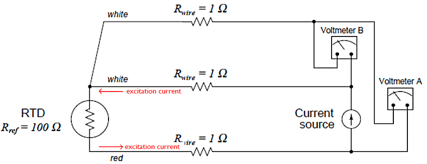 Figure 8 RTD connected to voltmeters in three-wire configuration
- In a three-wire RTD circuit, voltmeter “A” measures the voltage dropped across the RTD plus the voltage dropped across the bottom current-carrying wire. Voltmeter “B” measures just the voltage dropped across the top current-carrying wire. Assuming both current-carrying wires will have (very nearly) the same resistance, subtracting the indication of voltmeter “B” from the indication given by voltmeter “A” yields the voltage dropped across the RTD:
VRTD = Vmeter(A) - Vmeter(B)
Once again, RTD resistance is calculated from the RTD voltage and the known current source value using Ohm’s Law, just as it is in a 4-wire circuit.
If the resistances of the two current-carrying wires are precisely identical (and this includes the electrical resistance of any connections within those current-carrying paths, such as terminal blocks), the calculated RTD voltage will be the same as the true RTD voltage, and no wire-resistance error will appear. If, however, one of those current-carrying wires happens to exhibit more resistance than the other, the calculated RTD voltage will not be the same as the actual RTD voltage, and a measurement error will result.
Thus, we see that the three-wire RTD circuit saves us wire cost over a four-wire circuit, but at the “expense” of a potential measurement error. The beauty of the four-wire design was that wire resistances were completely irrelevant: a true determination of RTD voltage (and therefore RTD resistance) could be made regardless of how much resistance each wire had, or even if the wire resistances were different from each other. The error-cancelling property of the three-wire circuit, by contrast, hinges on the assumption that the two current-carrying wires have exactly the same resistance, which may or may not actually be true.
It should be understood that real three-wire RTD instruments do not employ direct-indicating voltmeters as shown in these simplified examples. Actual RTD instruments use either analogue or digital “conditioning” circuits to measure the voltage drops and perform the necessary calculations to compensate for wire resistance.
The voltmeters shown in the four-wire and three-wire diagrams serve only to illustrate the basic concepts, not to showcase practical instrument designs.
Self heating Error
- One problem inherent to both thermistors and RTDs is self-heating. In order to measure the resistance of either device, we must pass an electric current through it. Unfortunately, this results in the generation of heat at the resistance according to Joule’s Law:
P = 𝐼 2R
This dissipated power causes the thermistor or RTD to increase in temperature beyond its surrounding environment, introducing a positive measurement error. The effect may be minimized by limiting excitation current to a bare minimum, but this results in less voltage dropped across the device. The smaller the developed voltage, the more sensitive the voltage-measuring instrument must be to accurately sense the condition of the resistive element. Furthermore, a decreased signal voltage means we will have a decreased signal-to-noise ratio, for any given amount of noise induced in the circuit from external sources.
One clever way to circumvent the self-heating problem without diminishing excitation current to the point of uselessness is to pulse current through the resistive sensor and digitally sample the voltage only during those brief time periods while the thermistor or RTD is powered. This technique works well when we are able to tolerate slow sample rates from our temperature instrument, which is often the case because most temperature measurement applications are slow-changing by nature. The pulsed-current technique enjoys the further advantage of reducing power consumption for the instrument, an important factor in battery-powered temperature measurement applications
Figure 8 RTD connected to voltmeters in three-wire configuration
- In a three-wire RTD circuit, voltmeter “A” measures the voltage dropped across the RTD plus the voltage dropped across the bottom current-carrying wire. Voltmeter “B” measures just the voltage dropped across the top current-carrying wire. Assuming both current-carrying wires will have (very nearly) the same resistance, subtracting the indication of voltmeter “B” from the indication given by voltmeter “A” yields the voltage dropped across the RTD: VRTD = Vmeter(A) - Vmeter(B) Once again, RTD resistance is calculated from the RTD voltage and the known current source value using Ohm’s Law, just as it is in a 4-wire circuit.
If the resistances of the two current-carrying wires are precisely identical (and this includes the electrical resistance of any connections within those current-carrying paths, such as terminal blocks), the calculated RTD voltage will be the same as the true RTD voltage, and no wire-resistance error will appear. If, however, one of those current-carrying wires happens to exhibit more resistance than the other, the calculated RTD voltage will not be the same as the actual RTD voltage, and a measurement error will result.
Thus, we see that the three-wire RTD circuit saves us wire cost over a four-wire circuit, but at the “expense” of a potential measurement error. The beauty of the four-wire design was that wire resistances were completely irrelevant: a true determination of RTD voltage (and therefore RTD resistance) could be made regardless of how much resistance each wire had, or even if the wire resistances were different from each other. The error-cancelling property of the three-wire circuit, by contrast, hinges on the assumption that the two current-carrying wires have exactly the same resistance, which may or may not actually be true.
It should be understood that real three-wire RTD instruments do not employ direct-indicating voltmeters as shown in these simplified examples. Actual RTD instruments use either analogue or digital “conditioning” circuits to measure the voltage drops and perform the necessary calculations to compensate for wire resistance. The voltmeters shown in the four-wire and three-wire diagrams serve only to illustrate the basic concepts, not to showcase practical instrument designs. - RTDs are completely passive sensing elements, requiring the application of an externally-sourced electric current in order to function as temperature sensors. Thermocouples, however, generate their own electric potential. In some ways, this makes thermocouple systems simpler because the device receiving the thermocouple’s signal does not have to supply electric power to the thermocouple.
-
(Cont.)- Thermocouples were the first type of sensor used in non-contact pyrometers, and they still find application in modern versions of the same technology. Since the sensor does not become nearly as hot as the target object, the output of any single thermocouple junction at the sensor area will be quite small. For this reason, instrument manufacturers often employ a series-connected array of thermocouples called a thermopile to generate a stronger electrical signal.
The basic concept of a thermopile is to connect multiple thermocouple junctions in series so their voltages will add, Figure 13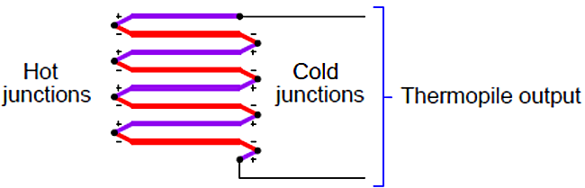 Figure 13. Thermopile
Examining the polarity marks of each junction (type E thermocouple wires are assumed in this example: chromel and constantan), we see that all the “hot” junctions’ voltages aid each other, as do all the “cold” junctions’ voltages. Like all thermocouple circuits, though, the each “cold” junction voltage opposes each the “hot” junction voltage. The example thermopile shown in this diagram, with four hot junctions and four cold junctions, will generate four times the potential difference that a single type E thermocouple hot/cold junction pair would generate, assuming all the hot junctions are at the same temperature and all the cold junctions are at the same temperature.
When used as the detector for a non-contact pyrometer, the thermopile is oriented so all the concentrated light falls on the hot junctions (the “focal point” where the light focuses to a small spot), while the cold junctions face away from the focal point to a region of ambient temperature. Thus, the thermopile acts like a multiplied thermocouple, generating more voltage than a single thermocouple junction could under the same temperature conditions.Distance considerations
- An interesting and useful characteristic of non-contact pyrometers is that their calibration does not depend on the distance separating the sensor from the target object’s surface. This is counterintuitive to anyone who has ever stood near an intense radiative heat source: standing in close proximity to a bonfire, for example, results in much hotter skin temperature than standing far away from it. Why wouldn’t a non-contact pyrometer register cooler target temperatures when it was far away, given the fact that infrared radiation from the object spreads out with increased separation distance? The fact that an infrared pyrometer does not suffer from this limitation is good for our purposes in measuring temperature, but it doesn’t seem to make sense at first.
One key to understanding this paradox is to quantify the bonfire experience, where perceived temperature falls off with increased distance. In physics, this is known as the inverse square law: the intensity of radiation falling on an object from a point-source decreases with the square of the distance separating the radiation source from the object. Backing away to twice the distance from a bonfire results in a four-fold decrease in received infrared radiation; backing way to three times the distance results in a nine-fold decrease in received radiation.
Placing a sensor at three integer distances (x, 2x, and 3x) from a radiation point-source results in relative power levels of 100%, 25% (one-quarter), and 11.1% (one-ninth) falling upon the sensor at those locations, respectively, Figure 14.
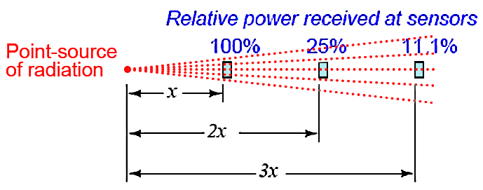 Figure 14. Relative power received from sensor as function of distance from a point-source
- This is a basic physical principle for all kinds of radiation, grounded in simple geometry. If we examine the radiation flux emanating from a point-source, we find that it must spread out as it travels in straight lines, and that the spreading-out happens at a rate defined by the square of the distance. An analogy for this phenomenon is to imagine a spherical latex balloon expanding as air is blown into it. The surface area of the balloon is proportional to the square of its radius. Likewise, the radiation flux emanating from a point-source spreads out in straight lines, in all directions, reaching a total area proportional to the square of the distance from the point (center). The total flux measured as a sphere will be the same no matter what the distance from the point-source, but the area it is divided over increases with the square of the distance, and so any object of fixed area backing away from a point-source of radiation encounters a smaller and smaller fraction of that flux.
Continues on next tab
Example 3: Logical AND Function (Contacts in Series)
- Figure shows an AND function.
- When Switches SW1 AND SW2 are closed IN1 AND IN2 contacts close energising the control relay RC1 turning ON the load.
- It is important to note that closing only one switch will not turn on the load.
Figure: Logical AND with PLC software
Example 4: Logical OR Function (Contacts in Parallel)
- Figure shows an OR function.
- When Switches Sw1 OR Sw2 are closed IN1 OR IN2 contacts close energising the control relay RC1 turning ON the load.
- It is important to note that closing only one switch is sufficient to turn on the load.
Figure: Logical OR with PLC software
Mechanical Switches
- The basic part of a limit switch is an electrical switch which is switched on or off by means of a plunger(Figure 21(A)), the movement of this plunger being controlled by the actuator head of the limit switch which transfers the external force and movement to it. Depending on the object and movement being detected, the actuator head can take a number of forms. A common form is a roller rotating an arm to move a plunger inside the switch to activate the switch contacts and having a spring return (Figure 21(B)).
The way in which the plunger moves when making the switch contacts and when breaking them is determined by springs to enable the switch to be slow or fast acting when making or breaking contacts. Figure 21. The basic form a limit switch: (A) the built-in switch with the contacts being switched by the movement of plunger, (B) a roller-actuated limit switch, rotation of the roller arm moving the plunger, and (C) a simple application of limit switches.
Example 7: Coil Feedback
- A control relay can be associated with a contact with the same label. When the control relay is energised, its associated contact changes state.
- Figure shows an example of this. When the switch is closed, IN1 contacts are closed and the output control relay RC1 is energised. As soon as the control relay RC1 is energised, its associated input contacts are also closed energising RC2.
- The load is therefore turned ON. Opening the switch will de-energise control relay RC1 hence opening contacts of RC1 and turning the load OFF.
Figure: Coil feedback system: Note hat RC1 is an internal (software) relay and not associated with a physical input or output
Example 8: Latch Circuit
- A latch circuit is used to hold a control relay energised even if the input contact which energised it turned off. An example of a latch circuit is shown in the figure below.
- When the switch is closed, IN1 contacts are closed and the relay coil RC1 is energised. The Load is turned ON and contacts of RC1 are also closed. Control relay RC1 is now also energised through the input contacts of RC1. If the switch is now opened, IN1 contacts will open, but control relay RC1 will remain energised through contacts RC1. The load therefore remains turned ON.
- The output is said to be LATCHED ON.
Figure: Latch Circuit and the corresponding PLC ladder diagram.Example 9: Breaking the Latch Circuit
- Figure shows how to break a latch circuit. When the switch Sw1 is closed momentarily, contact IN1 closes momentarily and control relay RC1 is latched on.
- To break this latch circuit, close switch Sw2 to open contacts IN2 de-energising control relay RC1 and hence opening input contacts RC1.

Figure: Latch Circuit and the corresponding PLC ladder diagram.
Example 10: Delay in Operation of an Output
- Figure shows a timer being used to delay turning on lamp 1 and delay turning off lamp 2.
- Timers normally open (NO) and normally closed (NC) contacts are connected to RC1 and RC2.
- Initially RC1 is de-energised and RC2 is energised. Hence, lamp 1 is off, lamp 2 is ON. When the switch is closed, IN1 contacts are closed energising T1. Timer T1 has a pre-set delay of 5 sec. 5 seconds after the timer is energised, its associated contacts change state. RC1 is energised and Lamp 1 is turned ON, RC2 is de-energised and Lamp 2 goes OFF. Opening the switch will reset the timer and its contacts back to their original de-energised states.
Figure: Using Timer in PLC
Example 11: Operating an Output for a Pre-set Time
- Figure shows how a PLC output can be turned ON for a pre-set time before being turned OFF.
- When the switch Sw 1 is closed, the timer T1 and the control relay RC1 are energised, turning the lamp ON. Five seconds later the timer contacts T1 open de-energising control relay RC1 turning OFF the lamp.
- [NOTE:] The contacts IN1 must be held closed to keep the timer energised during the delay period. Opening contacts IN1 reset the time delay back to the pre-set value and returns the contacts associated with the timer back to their de-energised state.

Figure: Using Timer in PLCExample 12: Sequencing outputs using timers
- The ladder diagram shows how to use 3 timers to repeatedly energise and de-energise control relays RC1, RC2 and RC3 one after the other as indicated in the timing diagram shown in the next slide.
- The sequencing starts when IN1 (push button with spring return) is momentarily pressed. This energise timer T1 and control relay RC1 for 5 seconds.
- When the 5 sec delay is completed, NC contacts of T1 is energised to open and control relay RC1 is de-energised. NO contacts of T1 closed to energise RC2 and T2.
- 5 seconds later NC contacts of T2 is opened and RC2 is de-energised and T2 resets itself. However NO contacts of T2 are closed to energise RC3 and start the timer T3. After 5 seconds T3 resets itself and start T1 again. External switch IN2 breaks all the latch circuit to stop the sequencing.

Figure: Sequencing with multiple timers
Example 12b: Timing diagram and the code for PLC

Non-contact temperature sensors
- Virtually any mass above absolute zero temperature emits electromagnetic radiation (photons, or light) as a function of that temperature. This basic fact makes possible the measurement of temperature by analysing the light emitted by an object. The Stefan-Boltzmann Law of radiated energy quantifies this fact, declaring that the rate of heat lost by radiant emission from a hot object is proportional to the fourth power of the absolute temperature: $$ \frac{dQ}{dt} = e \sigma AT ^4 $$ Where
$ \large \frac{dQ}{dt} $ = Radiant heat loss rate (Watts)
e = Emissivity factor (unitless)
$ \sigma $ = Stefan - Boltzmann constant (5.67x10⁻⁸ $ \large \frac{W}{m^2 K^4}$)
A = Surface Area (m2)
T = Absolute Temperature (K)
The primary advantage of non-contact thermometry (or pyrometry as high-temperature measurement is often referred) is rather obvious: with no need to place a sensor in direct contact with the process, a wide variety of temperature measurements may be made that are either impractical or impossible to make using any other technology.
A major disadvantage of non-contact thermometry is that it only reveals the surface temperature of an object. Sensing the thermal radiation emanated from a pipe, for instance, only tells you the surface temperature of that pipe and not the true temperature of the fluid within the pipe. Another example is when doctors use non-contact thermometry to assess irregularities in body temperature:
What they detect is just skin temperature. While it may be true that “hot spots” beneath the surface of an object may be detectable this way, it is only because the surface temperature of that object differs as a consequence of the hot spot(s) beneath. If a hotter-than-normal region inside of an object fails to transfer enough thermal energy to the surface to manifest as a hotter surface temperature, that region will be invisible to non-contact thermometry.Concentrating pyrometers
- A time-honoured design for non-contact pyrometers is to concentrate incident light from the surface of a heated object onto a small temperature-sensing element. A rise in temperature at the sensor reveals the intensity of the infrared optical energy falling upon it, which as discussed previously is a function of the target object’s surface temperature (absolute temperature to the fourth power), Figure 12
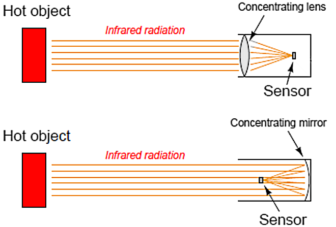 Figure 12. Designs of non-contact pyrometer
The fourth-power characteristic of Stefan-Boltzmann’s law means that a doubling of absolute temperature at the hot object results in sixteen times as much radiant energy falling on the sensor, and therefore a sixteen-fold increase in the sensor’s temperature rise over ambient. A tripling of target temperature (absolute) yields eighty one times as much radiant energy, and therefore an 81- fold increase in sensor temperature rise. This extreme nonlinearity limits the practical application of non-contact pyrometry to relatively narrow ranges of target temperature wherever good accuracy is required.
- Thermocouples were the first type of sensor used in non-contact pyrometers, and they still find application in modern versions of the same technology. Since the sensor does not become nearly as hot as the target object, the output of any single thermocouple junction at the sensor area will be quite small. For this reason, instrument manufacturers often employ a series-connected array of thermocouples called a thermopile to generate a stronger electrical signal.
-
Emissivity
- Aside from their inherent nonlinearity, perhaps the main disadvantage of non-contact temperature sensors is their inaccuracy. The emissivity factor (e) in the Stefan-Boltzmann equation varies with the composition of a substance, but beyond that there are several other factors (surface finish, shape, etc.) that affect the amount of radiation a sensor will receive from an object. For this reason, emissivity is not a very practical way to gauge the effectiveness of a non-contact pyrometer. Instead, a more comprehensive measure of an object’s “thermal-optical measurability” is emittance.
A perfect emitter of thermal radiation is known as a blackbody. Emittance for a blackbody is unity (1), while emittance figures for any real object is a value between 1 and 0. The only certain way to know the emittance of an object is to test that object’s thermal radiation at a known temperature. This assumes we have the ability to measure that object’s temperature by direct contact, which of course renders void one of the major purposes of non-contact thermometry: to be able to measure an object’s temperature without having to touch it. Not all hope is lost, though: all we have to do is obtain an emittance value for that object one time, and then we may calibrate any non-contact pyrometer for that object’s particular emittance so as to measure its temperature in the future without contact.
Beyond the issue of emittance, other idiosyncrasies plague non-contact pyrometers. Objects also have the ability to reflect and transmit radiation from other bodies, which taints the accuracy of any non-contact device sensing the radiation from that body. An example of the former is trying to measure the temperature of a silver mirror using an optical pyrometer: the radiation received by the pyrometer is mostly from other objects, merely reflected by the mirror. An example of the latter is trying to measure the temperature of a gas or a clear liquid, and instead primarily measuring the temperature of a solid object in the background (through the gas or liquid).
Nevertheless, non-contact pyrometers have been and will continue to be useful in specific applications where other, contact-based temperature measurement techniques are impractical.
Question #1 - When the temperature of an object is measured, in which case can the distance between the non-contact temperature sensor and the object be neglected?
Question #2 - Non-contact temperature sensors are widely used because of their:
Distance considerations (Cont.)
Figure 14. Relative power received from sensor as function of distance from a point-source
- If non-contact pyrometers really were “looking” at a point-source of infrared radiation, their signals would indeed decrease with distance. The saving grace here is that non-contact pyrometers are focused-optic devices, with a definite field of view, and that field of view should always be completely filled by the target object (assumed to be at a uniform temperature). As distance between the pyrometer and the target object changes, the cone-shaped field of view covers a surface area on that object proportional to the square of the distance. Backing the pyrometer away to twice the distance increases the viewing area on the target object by a factor of four; backing away to three times the distance increases the viewing area nine times, Figure 15.
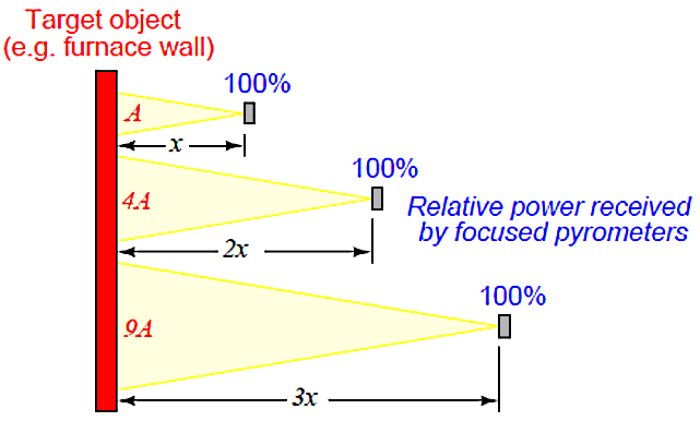 Figure 15. Relative power received from sensor as function of distance from a furnace wall type of object
So, even though the inverse square law correctly declares that radiation emanating from the hot wall (which may be thought of as a collection of point-sources) decreases in intensity with the square of the distance, this attenuation is perfectly balanced by an increased viewing area of the pyrometer. Doubling the separation distance does result in the flux from any given point on the wall spreading out by a factor of four, but the pyrometer now sees four times as many similar points on the wall as it did previously. So long as all the points within the field of view are uniform in temperature, the result is a perfect cancellation with the pyrometer providing the exact same temperature measurement at any distance from the target.
If the sensor’s field of view expands far enough to capture objects other than the one whose temperature we intend to measure, measurement errors will result. The sensor will now yield a weighted average of all objects within its field of view, and so it is important to ensure that field is limited to cover just the object we intend to measure.
Non-contact sensor fields-of-view are typically specified either as an angle, as a distance ratio, or both. For example, the following illustration shows a non-contact temperature sensor with a 5:1 (approximately 11°) field of view, Figure 16.
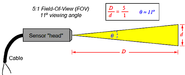 Figure 16. Non-contact sensor Field-of-View (FOV)
- Aside from their inherent nonlinearity, perhaps the main disadvantage of non-contact temperature sensors is their inaccuracy. The emissivity factor (e) in the Stefan-Boltzmann equation varies with the composition of a substance, but beyond that there are several other factors (surface finish, shape, etc.) that affect the amount of radiation a sensor will receive from an object. For this reason, emissivity is not a very practical way to gauge the effectiveness of a non-contact pyrometer. Instead, a more comprehensive measure of an object’s “thermal-optical measurability” is emittance.
-
(Cont.)- More examples of how thermal images can be used for measuring thermal efficiency and many similar parameters are shown on the following images.
The image below represents a home radiator heater. Clearly the temperature of the wall outside is 23.2°C, while the temperature at the heater itself reaches 70°C. If there are some obstructions in the thermal fluid flow, they would be visible on the image.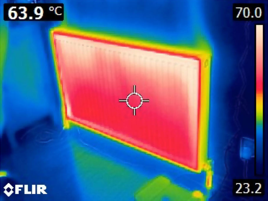
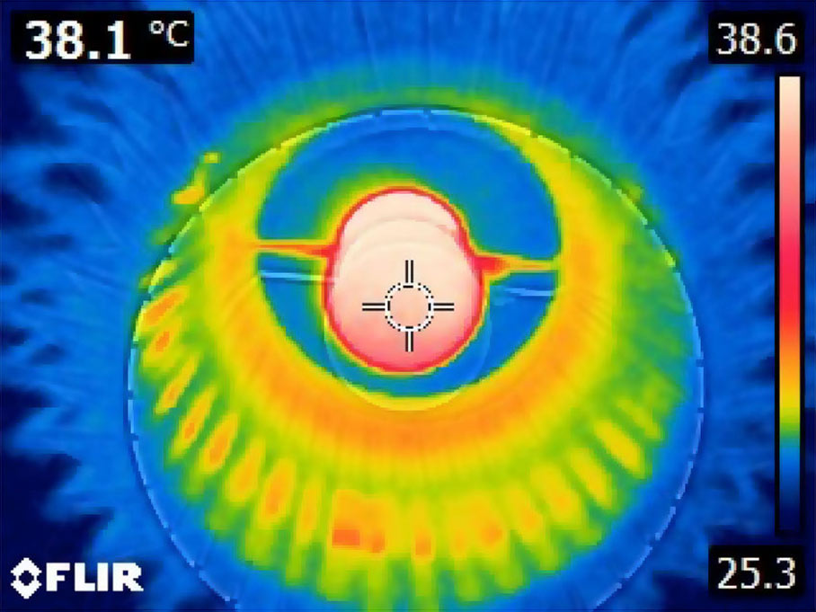
- The following two images clearly show how modern LED lighting is superior in the sense of energy efficiency compared to a linear tungsten halogen lamp.
The temperature in the tungsten lamp exceeds 280°C, while the temperature of the LED bulb hardly exceeds 38°C: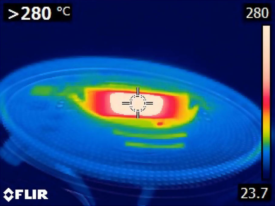
Example 3: Logical AND Function (Contacts in Series)
- Figure shows an AND function.
- When Switches SW1 AND SW2 are closed IN1 AND IN2 contacts close energising the control relay RC1 turning ON the load.
- It is important to note that closing only one switch will not turn on the load.
Figure: Logical AND with PLC software
Example 4: Logical OR Function (Contacts in Parallel)
- Figure shows an OR function.
- When Switches Sw1 OR Sw2 are closed IN1 OR IN2 contacts close energising the control relay RC1 turning ON the load.
- It is important to note that closing only one switch is sufficient to turn on the load.
Figure: Logical OR with PLC software
Example 5: Combined Logical AND and OR Functions (Contacts in Parallel & Series)
- Figure shows an example which uses combinations of normally open contacts, normally closed contacts, AND and OR functions.
- Closing Sw1 or Sw2 will close contacts IN1 OR IN2 respectively and the control relay RC1 will be energised through the normally closed contacts IN3, turning ON the load
- When Sw3 is closed IN3 contacts will open so the load will be turned OFF.
Figure: Combined Logical AND and OR with PLC software
Mechanical Switches
- Figure 27 shows the Hall effect principle. Current is passed through leads 1 and 2 of the element. The output ends will produce zero voltage when there is no transverse magnetic field passing through element. When there is a magnetic flux passing through the element, a voltage $V$ appears between output leads. This voltage is proportional to the current and field strength. The output voltage is represented in terms of element thickness, the flux intensity of the field, the current through the element, and the Hall coefficient as: $$ V = H \frac{IB}{T} $$ Where:
- $H$ = Hall coefficient, which can be defined as transverse electric potential gradient per unit magnetic field per unit current density. The units are Vm3/AWb.
- $I$ = current through the Element (A)
- $B$ = flux density (Wb/m2)
- $T$ = thickness of the element (m)
 Figure 27. Hall Effect Principle
Example 7: Coil Feedback
- A control relay can be associated with a contact with the same label. When the control relay is energised, its associated contact changes state.
- Figure shows an example of this. When the switch is closed, IN1 contacts are closed and the output control relay RC1 is energised. As soon as the control relay RC1 is energised, its associated input contacts are also closed energising RC2.
- The load is therefore turned ON. Opening the switch will de-energise control relay RC1 hence opening contacts of RC1 and turning the load OFF.
Figure: Coil feedback system: Note hat RC1 is an internal (software) relay and not associated with a physical input or output
Example 8: Latch Circuit
- A latch circuit is used to hold a control relay energised even if the input contact which energised it turned off. An example of a latch circuit is shown in the figure below.
- When the switch is closed, IN1 contacts are closed and the relay coil RC1 is energised. The Load is turned ON and contacts of RC1 are also closed. Control relay RC1 is now also energised through the input contacts of RC1. If the switch is now opened, IN1 contacts will open, but control relay RC1 will remain energised through contacts RC1. The load therefore remains turned ON.
- The output is said to be LATCHED ON.
Figure: Latch Circuit and the corresponding PLC ladder diagram.Example 9: Breaking the Latch Circuit
- Figure shows how to break a latch circuit. When the switch Sw1 is closed momentarily, contact IN1 closes momentarily and control relay RC1 is latched on.
- To break this latch circuit, close switch Sw2 to open contacts IN2 de-energising control relay RC1 and hence opening input contacts RC1.
Figure: Latch Circuit and the corresponding PLC ladder diagram.
Example 10: Delay in Operation of an Output
- Figure shows a timer being used to delay turning on lamp 1 and delay turning off lamp 2.
- Timers normally open (NO) and normally closed (NC) contacts are connected to RC1 and RC2.
- Initially RC1 is de-energised and RC2 is energised. Hence, lamp 1 is off, lamp 2 is ON. When the switch is closed, IN1 contacts are closed energising T1. Timer T1 has a pre-set delay of 5 sec. 5 seconds after the timer is energised, its associated contacts change state. RC1 is energised and Lamp 1 is turned ON, RC2 is de-energised and Lamp 2 goes OFF. Opening the switch will reset the timer and its contacts back to their original de-energised states.
Figure: Using Timer in PLC
Example 11: Operating an Output for a Pre-set Time
- Figure shows how a PLC output can be turned ON for a pre-set time before being turned OFF.
- When the switch Sw 1 is closed, the timer T1 and the control relay RC1 are energised, turning the lamp ON. Five seconds later the timer contacts T1 open de-energising control relay RC1 turning OFF the lamp.
- [NOTE:] The contacts IN1 must be held closed to keep the timer energised during the delay period. Opening contacts IN1 reset the time delay back to the pre-set value and returns the contacts associated with the timer back to their de-energised state.
Figure: Using Timer in PLCExample 12: Sequencing outputs using timers
- The ladder diagram shows how to use 3 timers to repeatedly energise and de-energise control relays RC1, RC2 and RC3 one after the other as indicated in the timing diagram shown in the next slide.
- The sequencing starts when IN1 (push button with spring return) is momentarily pressed. This energise timer T1 and control relay RC1 for 5 seconds.
- When the 5 sec delay is completed, NC contacts of T1 is energised to open and control relay RC1 is de-energised. NO contacts of T1 closed to energise RC2 and T2.
- 5 seconds later NC contacts of T2 is opened and RC2 is de-energised and T2 resets itself. However NO contacts of T2 are closed to energise RC3 and start the timer T3. After 5 seconds T3 resets itself and start T1 again. External switch IN2 breaks all the latch circuit to stop the sequencing.
Figure: Sequencing with multiple timers
Example 12b: Timing diagram and the code for PLC
Thermal Imaging
- A very useful application of non-contact sensor technology is thermal imaging, where a dense array of infrared radiation sensors provides a graphic display of objects in its view according to their temperatures. Each object shown on the digital display of a thermal imager is artificially coloured in the display on a chromatic scale that varies with temperature, hot objects typically registering as red tones and cold objects typically registering as blue tones. Thermal imaging is very useful in the electric power distribution industry, where technicians may inspect power line insulators and other objects at elevated potential for “hot spots” without having to make physical contact with those objects. Thermal imaging is also useful in performing “energy audits” of buildings and other heated structures, providing a means of revealing points of heat escape through walls, windows, and roofs. In such applications, relative differences in temperature are often more important to detect than specific temperature values. “Hot spots” readily appear on a thermal imager display, and may give useful data on the test subject even in the absence of accurate temperature measurement at any one spot.
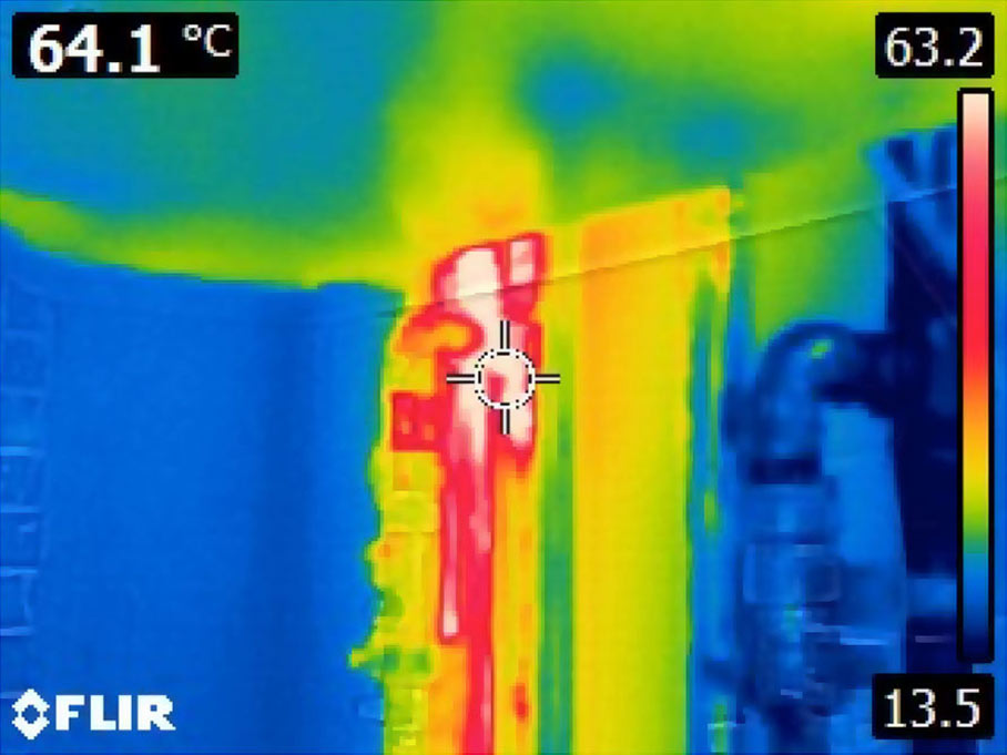
Again, it is important to stress that thermal imaging only provides an assessment of the object’s surface temperature, and not the temperature within that object. Variations in surface temperature detectable by thermal imaging are a secondary effect of temperature variations within the object, and as such may not accurately depict the true thermal gradient(s) within the object- A digital image taken with a thermal imaging instrument by maintenance personnel at a home boiler to inspect the temperatures of the water at the output. The hotspot of the temperature of 64.1°C is detected, and the colour scale in the range from dark blue (13.5°C) to white (63.2°C).
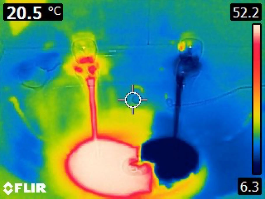
- Another thermal image (below) has been taken in a bathroom, where the bathroom sink was simultaneously filled with hot and cold water: In this particular image, the target, which is the circle in the image centre has temperature of 20.5°C, while we can clearly see the cold water, dark blue, temperature 6.3°C, and hot water at the temperature of 52.2°C.
- More examples of how thermal images can be used for measuring thermal efficiency and many similar parameters are shown on the following images.