-
Force, Torque and Acceleration Transducers
Control systems in automated manufacturing environments require extensive environmental information to make intelligent decisions. Such information relates to the tasks of material handling, machining, inspection, assembly, painting, etc. Assembly tasks and automated handling tasks require controlled operations like grasping, turning, inserting, aligning, orienting, and screwing. Every situation has somewhat different sensing requirements.
This module discusses some of the techniques used for force and torque sensing. A precise measurement of strain is an important consideration in measurement. Strain measurement is used as a secondary step in the measurement of many process variables, including flow, pressure, weight, and acceleration. Electrical-resistance strain gauges are widely used to measure strains due to force or torque. When a force is applied to a structure, it undergoes deformation. The gauge, which is bonded to the structure, is deformed by strain, and its electrical-resistance changes in a nearly linear fashion.
(Cont.)- And Poisson’s ratio is defined as:
$$ \nu = - frac{lateral \; strain}{longitudinal \; strain} = - \large \frac{\frac{\partial D}{D}}{\frac{\partial L}{L}}$$ $$ \frac{\partial D}{D} = - \nu \frac{\partial L}{L} $$
$$ \frac{1}{R} \frac{dR}{dS} = \frac{1}{L} \frac{\partial L}{\partial S} - \nu \frac{2}{L} \frac{\partial L}{\partial S} + \frac{1}{\rho} \frac{\partial \rho}{\partial S} $$ For small variations, the relationship in these equations can be written as:
$$ \frac{\Delta R}{R} = \frac{\Delta L}{L} + 2 \nu + \frac{\Delta \rho}{\rho} $$
Sensitivity or gauge factor, Gf, is defined as the ratio of unit change in resistance to unit change in length:
$$ G _f = \large \frac{\frac{\partial R}{R}}{\frac{\partial L}{L}}$$ And
$$ \frac{\Delta R}{R} = G _f \frac{\Delta L}{L} = G _f \varepsilon $$ Gauge factor can also be expresses as:
$$ G _f = \frac{\large\frac{\Delta R}{R}}{\large \frac{\Delta L}{L}} = 1 + 2 \nu + \large \frac{\frac{\Delta \rho}{\rho}}{\frac{\Delta L}{L}} \small = 1 + 2 \nu \; + \large \frac{\frac{\Delta \rho}{\rho}}{\varepsilon}$$ The change in resistivity occurs because of the piezoresistive effect, which is explained as an electrical resistance change which occurs when the material is mechanically deformed. In some cases, the effect is a source of error. If the change in resistivity or piezoresistive effect of the material is neglected, the gauge factor becomes:
$$ G _f = 1 + 2 \nu $$ The gauge factor gives an idea of the strain sensitivity of the gauge in terms of the change in resistance per unit strain. Although strain is a unitless quantity, it is a common practice to express strain as a ratio of two units as m/m. Poisson’s ratio for all metals is between 0 and 0.5. The gauge factor for metal can vary from 2 to 6. For semiconductors, it can vary between 40 to 200. Some common materials and their gauge factors are listed in Table:
Material Gauge Factor Nickel -12.6 Manganese +0.07 Nicrome +2.0 Constantan +2.1 Soft Iron +4.2 Carbon +20 Platinum +4.8
The gauge factor is normally supplied by the manufacturer from a calibration made of a number of gauges from a sample batch. The gauge factor for various metals ranges from -12 for nickel to +4 for soft iron. This indicates that changes in resistivity of a material could be quite significant while measurements are made.
Force, Torque and Acceleration Transducers (Cont.)
- If a piece of metal wire is stretched, not only does it get longer and thinner, but its resistance increases. The greater the strain experienced by the wire, the greater is the change in resistance.
There are a number of ways in which resistance can be changed by a physical phenomenon. The resistance, R, of a metal depends on its area, length, and electrical resistivity. It is possible to express the resistance of a conductor at a constant temperature, T, as:
$ R _0 = \large \frac{\rho l}{A_0} $Where:
ρ = resistivity (Ωm)
R0 = sample resistance (Ω)
l = length (m)
A0 = cross-sectional area, m2
Sensitivity of Resistive Transducers
- If a specimen is subjected to tension, causing an increase in length, its longitudinal dimension will increase, and its lateral dimension will decrease. If a resistance gauge made of this conducting material is subjected to a positive strain, its length increases while its cross-sectional area decreases. Since the resistance of the conductor is dependent on its length, cross-sectional area, and specific resistivity, the change in strain is due to the change in dimension or specific resistivity.For a circular wire of length, L; cross-sectional area, A; and diameter, D, the resistance of the wire before straining is: $$ R = \frac{\rho L}{A} $$ Let us subject the wire to tension which causes the strain. Tension increases length and reduces the diameter, which in turn reduces the area of cross section. Let the stress applied to the strain gauge be s in N/m2. Additional definitions are:
ΔL = change in length of wire
ΔA = change in area of cross-section
ΔD = change in diameter
ρ = resistivity
ν = Poisson’s ratio
$ \varepsilon $ = $ \large \frac{∆ L}{L} $ = Strain
In order to find how ΔR depends on the material physical quantities, the above equation for R is differentiated with respect to applied stress S: $$ \frac{dR}{dS} = \frac{\rho}{A} \frac{\partial L}{\partial S} - \frac{\rho L}{A ^2} \frac{\partial A}{\partial S} + \frac{L}{A} \frac{\partial \rho}{\partial S} $$ Dividing the last equation with the previous, we get: $$ \frac{1}{R} \frac{dR}{dS} = \frac{1}{L} \frac{\partial L}{\partial S} - \frac{1}{A} \frac{\partial A}{\partial S} + \frac{1}{\rho} \frac{\partial \rho}{\partial S} $$ The change in resistance is due to two items:
1. Unit change in length ΔL/L
2. Unit change in area ΔA/A
Since the area $ A = \large \frac{\pi D ^2}{4} $, we can write: $$ \frac{\partial A}{\partial S} = 2 \frac{\pi}{4} D \frac{\partial D}{\partial S} $$ And
$$ \frac{1}{A} \frac{\partial A}{\partial S} = \frac{2 \frac{\large \pi}{\large 4}D}{\frac{\large \pi}{\large 4}D^2} \frac{\partial D}{\partial S} = \frac{2}{D} \frac{\partial D}{\partial S} $$ This equation combined with an above gives:
$$ \frac{1}{R} \frac{dR}{dS} = \frac{1}{L} \frac{\partial L}{\partial S} - \frac{2}{D} \frac{\partial D}{\partial S} + \frac{1}{\rho} \frac{\partial \rho}{\partial S} $$
- And Poisson’s ratio is defined as:
Offset Voltage
- As shown in Figure 2, G is a null deflector that is used to compare potentials of point-B and D. The potential difference between points B and D is ΔV = VD - VB. If all the resistance values (R1, R2, R3, R4) chosen in the bridge circuit are same, then the voltage at points B and D are the same, ΔV will be zero, and the bridge is balanced. Let us consider R1 as the strain gauge. If R1 is strained, its resistance value changes, and the bridge becomes unbalanced, causing a nonzero ΔV. If any other resistance value is adjusted, the bridge can be brought back to a balanced condition. The adjusted value of any resistor needed to force ΔV to zero is equal to the strained value of the strain gauge. The current flowing through the bridge arms is computed as:
Current through ABC: I1 = $ \large \frac{V}{R_1 +R_4}$
Current through ABC: I2 = $ \large \frac{V}{R_2 +R_3}$
The voltage drop across R3 = R3I2, and the voltage drop across R4 = R4I1. The Voltage offset is given by: $$ \Delta V = V _D - V _B = \frac{R _3 V}{R _2 + R _3} - \frac{R _4 V}{R _1 + R _4} $$
$$ \Delta V = V \frac{R _3 R _1 - R _4 R _2}{(R _2 + R _3)(R _1 + R _4)} $$
In data acquisition systems where the ratio $ \large \frac{\Delta R}{R} $is small, the following method is suitable. Constant R supply voltage to the bridge is V, and ΔV is the output voltage.
Use R1 = R + ΔR and R2, R3, R4 equal to R. Therefore: $$ \Delta V = \bigg( \frac{R (R + \Delta R) - R^2}{(R + R)(R+ \Delta R + R)} \bigg) V $$
$$ \Delta V = \bigg( \frac{\Delta R}{4 R + 2 \Delta R} \bigg) V $$ If: $$ \frac{\Delta R}{R} = \delta ; \Delta V = \frac{\delta}{4 + 2 \delta} V $$ In systems, where the value $ \delta $ is small: $$ \Delta V = \frac{\delta}{4} V \; or \; \delta = \frac{4 \Delta V}{V} \; or \; \Delta R = \frac{4 R \Delta V}{V} $$Signal Enhancement
- Strain-gauge devices with signal-conditioning equipment are designed to balance the bridge automatically and provide the strain value in terms of microstrains. Data acquisition systems for force and strain measurement are programmed to provide the unbalanced offset voltage, which is proportional to the gauge resistance.
Figure 3 shows an arrangement of an instrumentation amplifier to be connected to the input channels of the data acquisition system.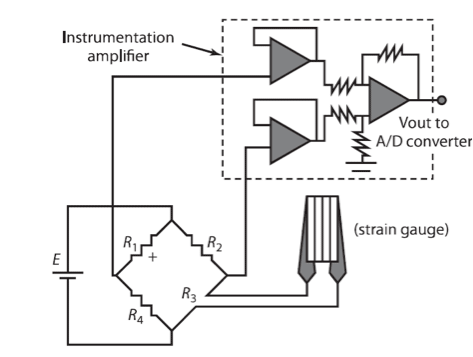 Figure 3. Bridge circuit with instrumentation amplifier
Possible Strain-Gauge Arrangement
When more than one arm of the bridge circuit contains strain transducers and their resistances change, the bridge output is due to the combined effect of these changes. More than one strain gauge, if suitably arranged, can lead to a higher signal-enhancement factor and a larger change in output voltage for a given strain.
For example, in Figure 2, R3 is the original strain gauge, and if we use R1 as another strain gauge placed in a location such that it has same strain as R3 the bridge output will be double the value obtained for a single gauge. In many experimental situations, there are areas of tension and compression in the same object with similar strain but of opposite sign. In such situations, care must be taken in arranging strain gauges in such a way that the adjacent arms of the bridge have strains of opposite nature.
In Figure 4, R1 measures changes due to axial tensile strain. In Figure 5 strain gauge R1 is bonded to the elastic member to measure axial tensile strain. R1 changes due to axial tensile strain. R2 measures changes due to transverse compressive strain. In the arrangement shown in Figure 6, both R1 and R3 are subjected to axial tensile strain of the same amount, and R1 and R3 form opposite arms of the bridge. This causes a signal enhancement factor of 2.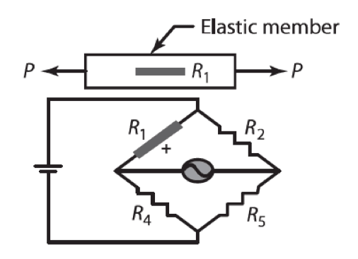 Figure 4. Possible arrangement of strain gauge to measure strain
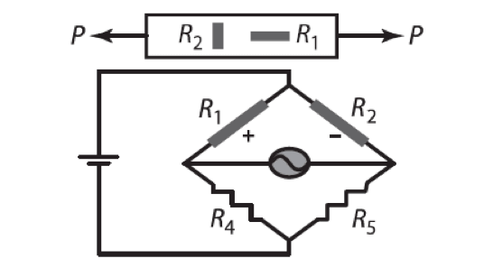 Figure 5. Possible arrangement of two strain gauges to measure strain
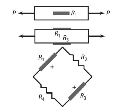 Figure 6. Possible arrangement of two strain gauges to measure tension
Continues on next tab
Strain Gauges
- A resistance strain gauge
consists of a grid of fine resistance wire of about 20 μm in diameter. The elements are formed on a backing film of electrically insulating material. Current strain gauges are manufactured from constantan foil, a copper-nickel alloy, or single-crystal semiconductor materials. The gauges are formed either mechanically or by photochemical etching. Strain-gauge transducers are of two types: unbonded and bonded.
Unbonded Strain Gauges
- In an unbonded strain gauge (Figure 1a), the resistance wire is stressed between the two frames. The first frame is called the fixed frame, and the second is called a moving frame. The wires in the unbonded gauges are connected such that the input motion of one frame stretches one set of wires and compresses another set of wires.
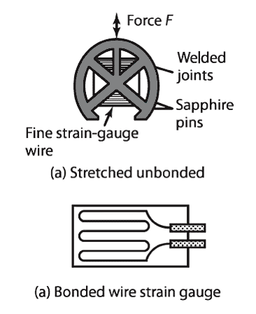 Figure 1. Strain Gauges
As an example, a 20 μm diameter wire is wound between insulated pins with one attached to a stationary frame and the other to a movable frame. For a particular stress input, the winding expe- riences either an increase or decrease in stress, resulting in a change in resistance. The output is con- nected to a Wheatstone bridge for measurement. With this type of strain gauge, measurement of small motions as small as a few microns can be made.
Bonded Strain Gauge
- Bonded strain-gauge transducers are widely used for measuring strain, force, torque, pressure, and vibration. The gauges have a backing material. Bonded strain gauges (Figure 1b) are made of metallic or semiconductor materials in the form of a wire gauge or thin metal foil. When the gauges are bonded to the surface, they undergo the same strain as that of the member surface. The coefficient of thermal expansion of the backing material should be matched to that of the wire.
Strain gauges are sensitive devices and are used with an electronic measuring unit. The strain gauge is normally made part of a Wheatstone bridge, so the change in its resistance due to strain either can be measured or used to produce an output, which can be displayed. Strains as low as a fraction of a micron can be measured using strain gauges. Following table presents characteristics of bonded strain gauges.
Material Gauge Factor Resistance Ω Resistance- Temperature Coefficient Ω/Ω/°C Comments Nichrome,Ni: 80%, Cr: 20% 2.5 -- 0.1x10⁻³ For use under 1200°C ConstantanNi: 45%, Cu: 55% 2.1 100 ±0.02x10⁻³ 400°C Platinum 4.8 50 4.0x10⁻³ For high temperature use Silicon -100 to +150 200 -- -- Nickel -12 -- 4.8x10⁻³ --
- For precise measurement, the strain gauges should have the following properties:
For precise measurement, the strain gauges should have the following properties.
The gauge characteristics are chosen so that the variation in resistance is a linear function of strain. If the gauges are used for dynamic measurements, the linearity should be maintained over the desired frequency range. High resistance of the strain gauge minimizes the effect of resistance variation in the signal-processing circuitry.
Strain gauges have a low temperature coefficient and absence of the hysteresis effect.
Bridge Circuit Arrangement
- The Wheatstone bridge circuit is used to measure the small changes in resistance that result in most strain-gauge applications. The change in resistance either can be measured or provided as an output that is processed by the computer. Figure 2 shows an arrangement of a bridge circuit. In the balanced bridge arrangement, strain-gauge resistance, R1, forms one arm of the Wheatstone bridge, while the remaining arms have resistances R2, R3, and R4. Between the points A and C of the bridge, there is a power supply; between points B and D, there is a precision galvanometer. The galvanometer gives an indication of the presence of current through that leg. For zero current to flow through the galvanometer, the points B and D must be at the same potential. The bridge is excited by the direct current source with voltage, V and Rg is the resistance in the galvanometer. The bridge is said to be balanced when there is no current flowing through the galvanometer.
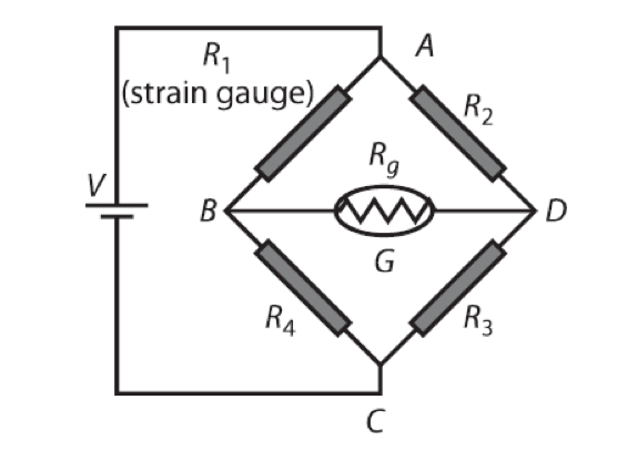 Figure 2. Bridge Circuit with Strain Gauge
The condition of balance is:
$$ \frac{R_1}{R_4} = \frac{R_2}{R_3} $$ If R1 changes due to strain, the bridge (which is initially in the balanced condition) becomes unbalanced. This may be balanced by changing R4 or R2. The change can be measured and used to indicate the change in R1. This procedure is useful for measuring static strains.
In the unbalanced bridge arrangement, the current through the galvanometer or the voltage drop across it is used to indicate the strain. This is useful for measuring dynamic as well as static strains.
Question #1 - 1. Strain Gauge is most commonly used for which physical quantity:
Question #2 - Which electrical parameter is measured in Strain Gauge
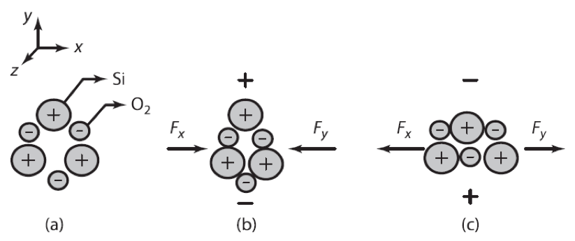
Figure 12. Differential arrangement of plates
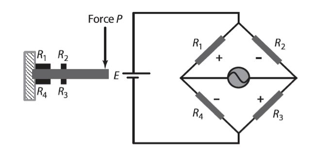
Figure: Output Module
- As shown in Figure 2, G is a null deflector that is used to compare potentials of point-B and D. The potential difference between points B and D is ΔV = VD - VB. If all the resistance values (R1, R2, R3, R4) chosen in the bridge circuit are same, then the voltage at points B and D are the same, ΔV will be zero, and the bridge is balanced. Let us consider R1 as the strain gauge. If R1 is strained, its resistance value changes, and the bridge becomes unbalanced, causing a nonzero ΔV. If any other resistance value is adjusted, the bridge can be brought back to a balanced condition. The adjusted value of any resistor needed to force ΔV to zero is equal to the strained value of the strain gauge. The current flowing through the bridge arms is computed as:
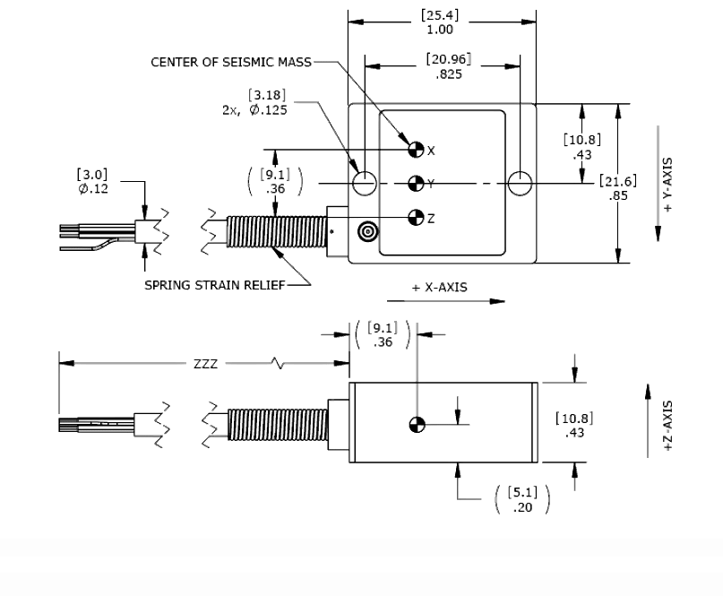
Acceleration Sensing using Strain Gauges
- Strain gauges are used in a variety of electrical transducer devices. Their advantages include ease of instrumentation, high accuracy, and excellent reliability. One of the most common configurations used in pressure, force, displacement, and acceleration transducers is the cantilever configuration with strain gauges mounted at the base, shown in Figure 10. A point mass of weight W is used as the acceleration-sensing element, and the cantilever (mounted with gauges) converts the inertial force into a strain.
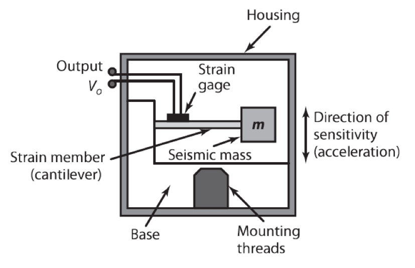 Figure 10. Acceleration Sensing
Figure 11 presents a photograph of a load cell being used in a force measurement application.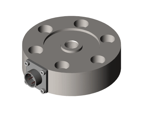
 Figure 11. Load Cell
Semiconductor Strain Gauges
- Semiconductor strain gauges are very useful in low strain applications. Use of semiconductor silicon has notably increased during the last few years. In a semiconductor gauge, the resistivity changes with strain as well as with physical dimensions. Changes in electron and hole mobility with changes in crystal structure as strain is applied results in larger gauge factors than possible with the metal gauges. Gauge factors of semiconductor gauges are between 50 and 200.
Semiconductor strain gauges physically appear as a band or strip of material with an electrical connection. The gauge is either bonded directly to the test element, or if encapsulated, it is attached by the encapsulation material. Signal conditioning is essentially a bridge circuit with temperature compensation.
There is also a need to linearize the output, because the basic characteristic of resistance verses strain is nonlinear. For good linearity of the output voltage with respect to strain, it is desirable to maintain a constant gauge current. This is accomplished by maintaining constant voltage excitation or by suitable modification, which produces constant current in the bridge arm in addition to constant voltage.
The benefits of semiconductor strain gauges are low power consumption and low heat generation. In addition, the mechanical hysteresis is negligible. The relation between the change in resistance and strain is approximately quadratic: $$ \delta = \frac{\Delta R}{R} = G _{f1} \varepsilon + G _{f2} \varepsilon ^2 $$ The resistance of semiconductor strain gauges varies from 1000 to 5000 Ω. They are usually made from p- or n-type silicon material.
Question #1 - Temperature has no influence on the work of Strain Gauge
Question #2 - The reliability of a strain gauges is poor:
Optical Proximity Sensors
- There are a variety of optical sensors that can be used to determine whether an object is present or not. Photoelectric switch devices can either operate as transmissive types where the object being detected breaks a beam of light, usually infrared radiation, and stops it reaching the detector (Figure 19(A)) or reflective types where the object being detected reflects a beam of light onto the detector (Figure 19(B)).
In both types the radiation emitter is generally a light-emitting diode (LED). The LED is a basic pn junction diode which emits light when suitable voltage is applied to it. The LED emits radiation which is reflected by the object. The reflected radiation is then detected by a phototransistor. In the absence of the object there is no detected reflected radiation; when the object is in the proximity, there is. The radiation detector might be a photodiode or a phototransistor, often a pair of transistors, known as a Darlington pair; using the pair increases the sensitivity.
Depending on the circuit used, the output can be made to switch to either high or low when light strikes the transistor. Such sensors are supplied as packages for sensing the presence of objects at close range, typically at less than about 5 mm.
Figure 19(C) shows a U-shaped form where the object breaks the light beam and so changes the response from a photodetector.
Another form of optical sensor is the pyroelectric sensor. Such sensors give a voltage signal when the infrared radiation falling on them changes, no signal being given for constant radiation levels. Lithium tantalate is a widely used pyroelectric material.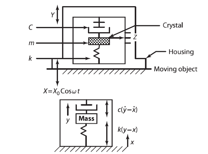
Figure 19. Photoelectric proximity sensors
Example 1: Normally Open Contacts
- Figure shows a practical example which uses normally open contacts in the ladder diagram
- When the switch is closed, $+24V$ is connected to IN1 of the PLC. This closes the contacts IN1 of the ladder diagram to energise control relay RC1 and hence turn load ON.
- If the switch is opened again, the contacts IN1 will spring open de-energising relay RC1 turning load OFF.
Figure: Normally Open contacts: The input contacts (IN1 etc) are not real contacts, they are part of the program.
Example 2: Normally Closed Contacts
- Figure shows a practical example which uses normally closed contacts in the ladder diagram
- Initially control relay RC1 is energised through normally closed contacts IN1.
- When the switch is closed, contacts IN1 will open de-energising control relay RC1 and switching OFF the load.
- When the switch is opened, contacts IN1 return to their normally closed state, hence RC1 is energised and the load is ON.
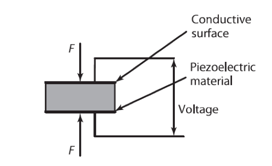
Figure: Figure: Normally Open contacts: The input contacts (IN1 etc) are not real contacts, they are part of the program.Possible Strain-Gauge Arrangement (Cont.)
- In the example shown in Figure 7, R1 has tensile strain, and R2 has compressive strain. R3 also has tensile strain, and R4 has compressive strain. Strain gauges R1, R2, R3 and R4 are bonded at the root of the cantilevers, where the bending stresses are maximum. In the arrangement shown in Figure 8 four active gauges are used with R2 and R4 arranged at right angles to R1 and R3 to produce a signal enhancement factor of 2(1 + $ \nu$ ), where $ \nu $ denotes Poisson’s ratio.
Figure 7. Cantilever deflection measurement
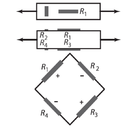 Figure 8 Alternative arrangements
In the arrangement shown in Figure 9, the strain gauges are arranged in such a way that R1 and R3 measure axial strains, while R2 and R4 measure the circumferential strains, which have strain of the opposite nature.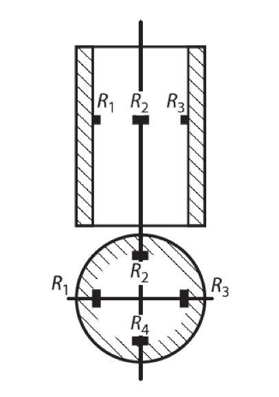 Figure 9. Hollow Cylinder with axial loading
Temperature effects in Strain Gauges
- The strain-gauge measuring environment is often influenced by temperature changes. The electrical resistivity of most alloys changes with temperature, increasing as temperature rises and decreasing as it falls. As shown in the previous table, metals used in strain gauges have a temperature coefficient (α0) of the order of 0.004/°C. The resistance at temperature T is given as:
RT = RT0 (1 + $\alpha _0 \Delta$ T)
Resistance change due to change in temperature ΔT is:
$\Delta R _T = $ = RT0 $\alpha _0 \Delta T $For example, if the temperature changes by one degree, the change in resistance is calculated as ΔT=1°, $ \alpha _0$ =0.004/°C, = RT0 =120 Ω, and ΔRT=0.48 Ω. When a strain gauge is bonded to the member being tested, its resistance will be affected by a change in temperature. This effect is independent of any strain applied to the gauge. The recording instrument cannot differentiate between the changes in the resistance due to temperature and strain. In addition, unless the coefficient of the linear expansion of the gauge is the same as that of the material to which it is bonded, the temperature change during measurement also will be a source of false strain due to differential expansion.Temperature Compensation
- Temperature compensation is achieved in two manners:
1. Using a dummy gauge.
2. Using more than one active gauge with proper arrangement of gauges.
If active and dummy gauges are mounted on the adjacent arms of a bridge, variation in temperature will not affect the bridge. The active gauge is subjected to strain as well as temperature change, while the dummy gauge is subjected to temperature change only. Since active and dummy gauges form adjacent arms of the bridge, the output due to temperature change is zero, as both active and dummy gauges change identically due to temperature. Furthermore, it is desirable to choose a gauge material with a coefficient of thermal expansion very close to that of the material under test.
Since it is inconvenient to calculate and apply temperature correction after the measurement is made, the temperature compensation can be made in the experimental setup itself. The gauges are suitably arranged so that adjacent arms have strains of opposite nature. This procedure ensures signal enhancement as well as temperature compensation.
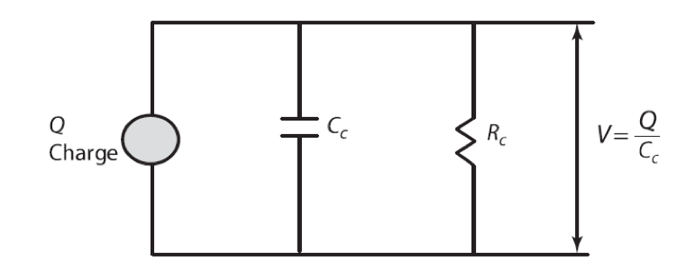
Figure 15. The rotating wheel of the absolute encoder. Note that though the normal form of binary code is shown in the figure, in practice a modified form of binary code called the Gray code is generally used. This code, unlike normal binary, has only one bit changing in moving from one number to the next. Thus we have the sequence 0000, 0001, 0011, 0010, 0011, 0111, 0101, 0100, 1100, 1101, 1111- Strain gauges are used in a variety of electrical transducer devices. Their advantages include ease of instrumentation, high accuracy, and excellent reliability. One of the most common configurations used in pressure, force, displacement, and acceleration transducers is the cantilever configuration with strain gauges mounted at the base, shown in Figure 10. A point mass of weight W is used as the acceleration-sensing element, and the cantilever (mounted with gauges) converts the inertial force into a strain.
(Cont.)- The piezoelectric effect is reversible. If a varying potential is applied to the proper axis of the crystal, it changes the dimension of the crystal, thereby deforming it. A piezoelectric element used for converting mechanical motion to electrical signals is thought of as both a charge generator and a capacitor. This charge appears as a voltage across the electrodes. The magnitude and polarity of the induced surface charges are proportional to the magnitude and direction of the applied force. For the arrangements shown in Figure 13 and 14, the charge generated, Q, is defined as:
Q = dF (Longitudinal effect)
Q = dF $ \frac{a}{b} $(Transverse effect)
Figure 13. Longitudinal effect
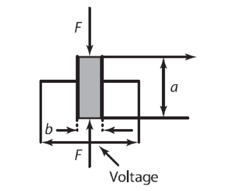 Figure 14 Transverse effect
Here d is the piezoelectric coefficient of the material. It is also known as the charge sensitivity factor of the crystal. For a typical quartz crystal, d=2.3x10⁻¹² C/N (Coulumbs pre Newton) or 2.3 pC/N (picocoulumbs per Newton).
If the ratio of a/b is greater than one, the transverse effect produces more charge than the longitudinal effect. The force, F, results in a change in thickness of the crystal. If the original thickness of the crystal is t and Δt is the change in thickness due to the applied force, Young’s modulus, E, can be expressed as the ratio of stress and strain: $$ Young’s \; Modulus: \; E = \frac{Strain}{Stress} = \frac{\large \frac{F}{A}}{\large \frac{\Delta t}{t}} = \frac{Ft}{A \Delta t} $$ Rewriting the expression, we have: $$ F = \frac{AE}{t} \Delta t $$ Where:
A = area of the crystal, m2
t = thickness of the crystal, m
Example 3: Logical AND Function (Contacts in Series)
- Figure shows an AND function.
- When Switches SW1 AND SW2 are closed IN1 AND IN2 contacts close energising the control relay RC1 turning ON the load.
- It is important to note that closing only one switch will not turn on the load.
Figure: Logical AND with PLC software
Example 4: Logical OR Function (Contacts in Parallel)
- Figure shows an OR function.
- When Switches Sw1 OR Sw2 are closed IN1 OR IN2 contacts close energising the control relay RC1 turning ON the load.
- It is important to note that closing only one switch is sufficient to turn on the load.
Figure: Logical OR with PLC software
Example 5: Combined Logical AND and OR Functions (Contacts in Parallel & Series)
- Figure shows an example which uses combinations of normally open contacts, normally closed contacts, AND and OR functions.
- Closing Sw1 or Sw2 will close contacts IN1 OR IN2 respectively and the control relay RC1 will be energised through the normally closed contacts IN3, turning ON the load
- When Sw3 is closed IN3 contacts will open so the load will be turned OFF.
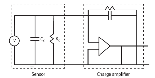
Figure: Combined Logical AND and OR with PLC software
Mechanical Switches
- The basic part of a limit switch is an electrical switch which is switched on or off by means of a plunger(Figure 21(A)), the movement of this plunger being controlled by the actuator head of the limit switch which transfers the external force and movement to it. Depending on the object and movement being detected, the actuator head can take a number of forms. A common form is a roller rotating an arm to move a plunger inside the switch to activate the switch contacts and having a spring return (Figure 21(B)).
The way in which the plunger moves when making the switch contacts and when breaking them is determined by springs to enable the switch to be slow or fast acting when making or breaking contacts. Figure 21. The basic form a limit switch: (A) the built-in switch with the contacts being switched by the movement of plunger, (B) a roller-actuated limit switch, rotation of the roller arm moving the plunger, and (C) a simple application of limit switches.
Example 8: Latch Circuit
- A latch circuit is used to hold a control relay energised even if the input contact which energised it turned off. An example of a latch circuit is shown in the figure below.
- When the switch is closed, IN1 contacts are closed and the relay coil RC1 is energised. The Load is turned ON and contacts of RC1 are also closed. Control relay RC1 is now also energised through the input contacts of RC1. If the switch is now opened, IN1 contacts will open, but control relay RC1 will remain energised through contacts RC1. The load therefore remains turned ON.
- The output is said to be LATCHED ON.
Figure: Latch Circuit and the corresponding PLC ladder diagram.Example 9: Breaking the Latch Circuit
- Figure shows how to break a latch circuit. When the switch Sw1 is closed momentarily, contact IN1 closes momentarily and control relay RC1 is latched on.
- To break this latch circuit, close switch Sw2 to open contacts IN2 de-energising control relay RC1 and hence opening input contacts RC1.

Figure: Latch Circuit and the corresponding PLC ladder diagram.
Example 10: Delay in Operation of an Output
- Figure shows a timer being used to delay turning on lamp 1 and delay turning off lamp 2.
- Timers normally open (NO) and normally closed (NC) contacts are connected to RC1 and RC2.
- Initially RC1 is de-energised and RC2 is energised. Hence, lamp 1 is off, lamp 2 is ON. When the switch is closed, IN1 contacts are closed energising T1. Timer T1 has a pre-set delay of 5 sec. 5 seconds after the timer is energised, its associated contacts change state. RC1 is energised and Lamp 1 is turned ON, RC2 is de-energised and Lamp 2 goes OFF. Opening the switch will reset the timer and its contacts back to their original de-energised states.
Figure: Using Timer in PLC
Example 11: Operating an Output for a Pre-set Time
- Figure shows how a PLC output can be turned ON for a pre-set time before being turned OFF.
- When the switch Sw 1 is closed, the timer T1 and the control relay RC1 are energised, turning the lamp ON. Five seconds later the timer contacts T1 open de-energising control relay RC1 turning OFF the lamp.
- [NOTE:] The contacts IN1 must be held closed to keep the timer energised during the delay period. Opening contacts IN1 reset the time delay back to the pre-set value and returns the contacts associated with the timer back to their de-energised state.

Figure: Using Timer in PLCExample 12: Sequencing outputs using timers
- The ladder diagram shows how to use 3 timers to repeatedly energise and de-energise control relays RC1, RC2 and RC3 one after the other as indicated in the timing diagram shown in the next slide.
- The sequencing starts when IN1 (push button with spring return) is momentarily pressed. This energise timer T1 and control relay RC1 for 5 seconds.
- When the 5 sec delay is completed, NC contacts of T1 is energised to open and control relay RC1 is de-energised. NO contacts of T1 closed to energise RC2 and T2.
- 5 seconds later NC contacts of T2 is opened and RC2 is de-energised and T2 resets itself. However NO contacts of T2 are closed to energise RC3 and start the timer T3. After 5 seconds T3 resets itself and start T1 again. External switch IN2 breaks all the latch circuit to stop the sequencing.

Figure: Sequencing with multiple timers
Example 12b: Timing diagram and the code for PLC

Tactile Sensors
- Tactile sensors are used in many applications ranging from fruit picking to monitoring human prosthetic implants; however, the major area of application is in the biomedical field. Tactile sensors are used for the following:
Other areas of application include the field of robotics, where tactile sensors can be placed on the gripper of the manipulator to provide feedback information from the workpiece. Besides being used as a touch sensor, gripping force sensors detect the force with which the object is gripped, pressure sensors detect the pressure applied to the object, and slip sensors can detect if the object is slipping. In addition, other industrial applications of the tactile sensors include the study of forces developed by fastening devices.Study the forces developed by the human foot during motion.Study the forces developed during various types of hand functions.Monitor the artificial knee and sense the forces developed.
A tactile sensing system has the ability to detect the following.
1. Presence of a part2. Part shape, location, and orientation3. Contact pressure distribution4. Force magnitude and direction
The major components of tactile sensors include:Touch surfaceTransducerStructure and control interface
Some tactile sensors are designed using piezoelectric films. Piezoelectric (Piezo) film consists of polyvinylidene fluoride (PVDF) that has undergone special processing to enhance its piezoelectric properties. Piezo film develops an electrical charge proportional to induced mechanical stress or strain. As a result, it produces a response proportional to the rate of stress rather than to the stress magnitude. This sensor is passive—that is, its output signal is generated by the piezoelectric film without the need for an excitation signal. The piezoelectric tactile sensor can be fabricated with the PVDF film strips imbedded into a rubber skin. To measure surface vibration, the film is bonded to the surface. As the surface vibrates, it stretches the surface in a cyclical manner, generating a volt- age. Piezo-film voltage output is relatively high.
A resistive tactile sensor known as a force sensing resistor (FSR) can be fabricated using material whose electrical conductivity changes with strain. FSR consists of a material whose resistance changes with applied pressure. Such materials are known as conductive elastomers fabricated of silicone rubber, polyurethane, and other compounds. The basic operating principle of elastomeric tactile sensors is based either on varying the contact area when the elastomer is squeezed between two conductive plates or on changing the thickness. When the external force varies the contact area at the interface of the elastomer, changes result in a reduction of electrical resistance. Compared with a strain gauge, the FSR has a much wider dynamic range. Miniature tactile sensors are used extensively in robotic applications where good spatial resolution, high sensitivity, and wide dynamic range are required.Piezoelectric Transducers
- Piezoelectric transducers depend upon the characteristics of certain materials that are capable of generating electric voltage when they deform. Piezoelectric materials, when subjected to mechanical force or stress along specific planes, generate electric charge. The property of generating an electric charge when deformed makes piezoelectric materials useful as primary sensors in instrumentation.
The best-known natural material is quartz crystal (SiO2). Rochelle salt is also considered a natural piezoelectric material. Artificial materials using ceramics and polymers, such as PZT (lead zirconium titanate), PVDF (polyvinylidene fluoride), BaTio3 (barium titanate), and LS (Lithium Sulfate) also exhibit the piezoelectric phenomenon.Piezoelectric Effect
- A piezoelectric material such as a quartz crystal can be cut along its axes in x, y, and z directions. Figure 12 shows a view along the z-axis. In a single-crystal cell, there are three atoms of silicon and six atoms of oxygen. Oxygen atoms are lumped in pairs. Each silicon atom carries four positive charges, and oxygen atoms carry two negative charges. A pair of oxygen atoms carries four negative charges. When there is no external force applied on the quartz crystal, the quartz cell is electrically neutral.
Figure 12. Piezoelectric effect in a crystal
- When compressive forces are applied along the x-axis, as shown in Figure 12(b), the hexagonal lattices become deformed. The forces shift the atoms in the crystal in such a manner that positive charges are accumulated at the silicon atom side and negative charges at the oxygen pair side. The crystal tends to exhibit electric charges along the y-axis. On the other hand, if the crystal is subjected to tension along the x-axis, as in Figure 12(c), a charge of opposite polarity is produced along the y-axis. To transmit the charge which has been developed, conductive electrodes are applied to the crystal at the opposite side of the cut.
- The piezoelectric effect is reversible. If a varying potential is applied to the proper axis of the crystal, it changes the dimension of the crystal, thereby deforming it. A piezoelectric element used for converting mechanical motion to electrical signals is thought of as both a charge generator and a capacitor. This charge appears as a voltage across the electrodes. The magnitude and polarity of the induced surface charges are proportional to the magnitude and direction of the applied force. For the arrangements shown in Figure 13 and 14, the charge generated, Q, is defined as:
Equivalent Circuit of a Piezoelectric Transducer
- The dynamic properties of a piezoelectric transducer can be represented by an equivalent circuit derived from the electrical and mechanical parameters of the transducer. The basic equivalent circuit is shown in Figure 15. The charge generated, Q, is across the capacitance Cc, and its leakage resistance is Rc. The charge source can be replaced by a voltage source, as per for following equation and drawn in series with a capacitance Cc and resistance Rc: $$ V = \frac{Q}{C} = \frac{dF}{C _c} $$
Figure 15. Piezoelectric transducer equivalent circuit
When the piezoelectric crystal is coupled with leads and cables as well as a readout device, the voltage depends not only on the element but also on the capacitance of cables, charge amplifier, and display. The total capacitance is expressed as:
CT = CC + Ccable + C display
A typical arrangement is shown in Figure 16, where the sensing element and charge amplifiers are presented.
Figure 16. Charge amplifier for piezoelectric transducer
The feedback resistance of the charge amplifier is kept high so that this circuit draws very low current and produces a voltage output that is proportional to the charge. Figure 17 shows the piezoelectric crystal interface, and the combined equivalent circuit is shown in Figure 18.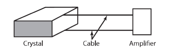 Figure 17. Piezoelectric crystal interface
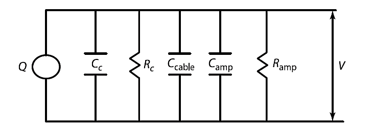 Figure 18. Combined equivalent circuit
Example 3: Logical AND Function (Contacts in Series)
- Figure shows an AND function.
- When Switches SW1 AND SW2 are closed IN1 AND IN2 contacts close energising the control relay RC1 turning ON the load.
- It is important to note that closing only one switch will not turn on the load.
Figure: Logical AND with PLC software
Example 4: Logical OR Function (Contacts in Parallel)
- Figure shows an OR function.
- When Switches Sw1 OR Sw2 are closed IN1 OR IN2 contacts close energising the control relay RC1 turning ON the load.
- It is important to note that closing only one switch is sufficient to turn on the load.
Figure: Logical OR with PLC software
Example 5: Combined Logical AND and OR Functions (Contacts in Parallel & Series)
- Figure shows an example which uses combinations of normally open contacts, normally closed contacts, AND and OR functions.
- Closing Sw1 or Sw2 will close contacts IN1 OR IN2 respectively and the control relay RC1 will be energised through the normally closed contacts IN3, turning ON the load
- When Sw3 is closed IN3 contacts will open so the load will be turned OFF.
Figure: Combined Logical AND and OR with PLC software
Mechanical Switches
- Figure 27 shows the Hall effect principle. Current is passed through leads 1 and 2 of the element. The output ends will produce zero voltage when there is no transverse magnetic field passing through element. When there is a magnetic flux passing through the element, a voltage $V$ appears between output leads. This voltage is proportional to the current and field strength. The output voltage is represented in terms of element thickness, the flux intensity of the field, the current through the element, and the Hall coefficient as: $$ V = H \frac{IB}{T} $$ Where:
- $H$ = Hall coefficient, which can be defined as transverse electric potential gradient per unit magnetic field per unit current density. The units are Vm3/AWb.
- $I$ = current through the Element (A)
- $B$ = flux density (Wb/m2)
- $T$ = thickness of the element (m)
 Figure 27. Hall Effect Principle
Example 8: Latch Circuit
- A latch circuit is used to hold a control relay energised even if the input contact which energised it turned off. An example of a latch circuit is shown in the figure below.
- When the switch is closed, IN1 contacts are closed and the relay coil RC1 is energised. The Load is turned ON and contacts of RC1 are also closed. Control relay RC1 is now also energised through the input contacts of RC1. If the switch is now opened, IN1 contacts will open, but control relay RC1 will remain energised through contacts RC1. The load therefore remains turned ON.
- The output is said to be LATCHED ON.
Figure: Latch Circuit and the corresponding PLC ladder diagram.Example 9: Breaking the Latch Circuit
- Figure shows how to break a latch circuit. When the switch Sw1 is closed momentarily, contact IN1 closes momentarily and control relay RC1 is latched on.
- To break this latch circuit, close switch Sw2 to open contacts IN2 de-energising control relay RC1 and hence opening input contacts RC1.
Figure: Latch Circuit and the corresponding PLC ladder diagram.
Example 10: Delay in Operation of an Output
- Figure shows a timer being used to delay turning on lamp 1 and delay turning off lamp 2.
- Timers normally open (NO) and normally closed (NC) contacts are connected to RC1 and RC2.
- Initially RC1 is de-energised and RC2 is energised. Hence, lamp 1 is off, lamp 2 is ON. When the switch is closed, IN1 contacts are closed energising T1. Timer T1 has a pre-set delay of 5 sec. 5 seconds after the timer is energised, its associated contacts change state. RC1 is energised and Lamp 1 is turned ON, RC2 is de-energised and Lamp 2 goes OFF. Opening the switch will reset the timer and its contacts back to their original de-energised states.
Figure: Using Timer in PLC
Example 11: Operating an Output for a Pre-set Time
- Figure shows how a PLC output can be turned ON for a pre-set time before being turned OFF.
- When the switch Sw 1 is closed, the timer T1 and the control relay RC1 are energised, turning the lamp ON. Five seconds later the timer contacts T1 open de-energising control relay RC1 turning OFF the lamp.
- [NOTE:] The contacts IN1 must be held closed to keep the timer energised during the delay period. Opening contacts IN1 reset the time delay back to the pre-set value and returns the contacts associated with the timer back to their de-energised state.
Figure: Using Timer in PLCExample 12: Sequencing outputs using timers
- The ladder diagram shows how to use 3 timers to repeatedly energise and de-energise control relays RC1, RC2 and RC3 one after the other as indicated in the timing diagram shown in the next slide.
- The sequencing starts when IN1 (push button with spring return) is momentarily pressed. This energise timer T1 and control relay RC1 for 5 seconds.
- When the 5 sec delay is completed, NC contacts of T1 is energised to open and control relay RC1 is de-energised. NO contacts of T1 closed to energise RC2 and T2.
- 5 seconds later NC contacts of T2 is opened and RC2 is de-energised and T2 resets itself. However NO contacts of T2 are closed to energise RC3 and start the timer T3. After 5 seconds T3 resets itself and start T1 again. External switch IN2 breaks all the latch circuit to stop the sequencing.
Figure: Sequencing with multiple timers
Example 12b: Timing diagram and the code for PLC
Piezoelectric Output
- From the previous equations we have: $$ Charge \; Q = \frac{dAE \Delta t}{t} C $$ The charge at the electrodes the voltage: $$ V = \frac{Q}{C} $$ The capacitance of the piezoelectric material between two electrodes is: $$ C = \varepsilon \frac{A}{t} = \varepsilon _0 \varepsilon _r \frac{A}{t} $$ Here $ \varepsilon _r $ is the dielectric constant (permittivity) of the material, and $ \varepsilon _0 $ is that for free space. Thus: $$ V = \frac{Q}{C} = \frac{dF}{\varepsilon _r \varepsilon _0 \large \frac{A}{t}} = \frac{dtF}{\varepsilon _r \varepsilon _0 A} $$ Expressing g as the crystal voltage sensitivity factor, the voltage can be written as:
g = $ \frac{\large d}{\large \varepsilon _r \varepsilon _0} Vm/N $
Also, g = $ \large \frac{V}{tP} = \frac{V/t}{P} $ where V/t is the electrical field strength and P is the pressure or stress.
The following table presents the basic properties and characteristics of typical piezoelectric materials:
Material Density(x 103 kg/m3) Permittivity
εrYoung’s Modulus E(x1010N/m2) Piezoelectric charge sensitivity d(pC/N) Quartz (SiO2) 2.65 4.5 7.7 2.3 Barium Titanate BaTiO3 5.8 1700 6.7 140 PZT 7.5 1200 8.3 110 PVDF 1.78 12 0.3 20 to 30 (based on crystal axes)
- Piezoelectric materials are used in a variety of applications where force, pressure, acceleration, and vibration measurements are taken. The major application of the piezoelectric sensor is in situations where the charge does not have much time to leak off. It is also used as the sensor in ceramic- or crystal-type pick ups, where the needle causes distortion of the crystal and the voltages generated are amplified by charge amplifiers, which have the additional capacity of reducing loading effects on piezoelectric transducers.
Sensitivity, natural frequency, nonlinearity, hysteresis, and temperature effects are the primary considerations when selecting piezoelectric transducers. Piezoelectric pressure sensors are used for the measurement of rapidly varying pressures as well as shock pressures. Sensors made of quartz materials generally exhibit stable frequency response from 1 Hz to 20 kHz—the natural frequency being of the order of 50 kHz. Quartz crystals can be used over a temperature range of -185 to +288°C compared to ceramic devices, which are limited to -185 to +100 °C.
Velocity Measurement by Piezoelectric Transducer
It is possible to measure velocity by first converting the velocity into a force using a viscous damping element and then measuring the resulting force with a PZT sensor. If acceleration data is available through an accelerometer, the velocity is obtained by integrating this device. Velocity transducers are constructed using piezo- electric accelerometers and integrating amplifiers. Double integration provides displacement information. The principle of piezoelectric velocity transducer is illustrated in Figure 20.
Figure 20. Velocity transducerAnalogy Equations
- Using mathematical models, solutions of equations describing one physical form can be applied to analogous systems in other fields. Using mechanical elements (such as inertial elements, spring, and damper), a mechanical system can be analysed. C, L, and R, represent mechanical parameters of compliance, mass, and viscous resistance of the element, respectively. The mechanical analogy in terms of displacement can be expressed as: $$ F = m \frac{d ^2 x}{dt ^2} + c \frac{dx}{dt} + \frac{x}{\large \frac{1}{k}}$$ $$ v = \frac{dx}{dt} $$ $$ F = m \frac{dv}{dt} + cv + \frac{1}{\large \frac{1}{k}} \int vdt $$ Differential equations in terms of current and velocity are also developed. R, L, and C, represent the viscous resistance of an element, mass, and parameters of mechanical parameters of compliance. In a R-L-C series electrical network, the applied voltage equals the drop across the resistor, plus the drop across the inductor, plus the drop across the capacitor. $$ Electrical:= R i + L \frac{di}{dt} + \frac{1}{C} \int idt $$ The configuration of the piezoelectric element is an important consideration in the industrial use of these elements. The shape of the element could be a disc, plate, or in tubular form. It may be operated under normal, transverse, or shear modes. For example, a small piezoelectric transducer 4 mm in diameter and 10 mm long weighs around 2 grams, operates at 177 °C, and has voltage sensitivity of 0.1 mV/N.
Acceleration Measurement by Piezoelectric Transducer
- The piezoelectric accelerometer is constructed as follows. It consists of a housing and contains a mass attached to the mechanical axis of the crystal. The piezoelectric element in the form of a cylinder is first bonded to a central pillar. Then a cylinder mass is bonded to the outside of the PZT element. Acceleration in the direction of the cylinder axis causes a shear force on the element, which provides its own spring force. The acceleration of the piezoelectric material generates electric potential when subjected to mechanical strain along a predetermined axis. The initial calibrating force is predetermined between the mass and spring using a preloaded spring.
As the housing of the accelerometer is subjected to vibrations, the force exerted on the piezoelectric element by the mass is altered. The charge generated on the crystal is sensed using a charge amplifier. A force F applied to the crystal develops a charge, Q = dF. When a varying acceleration is applied to the mass crystal assembly, the crystal experiences a varying force:
F = ma
Q = dF = dma$$ V = \frac{dF}{C} = \frac{dma}{C} $$ Here a is the acceleration and V is the voltage produced. Thus, the output is a measure of the acceleration.
Figure 19. Piezoelectric accelerometer
Because of the high stiffness of the piezoelectric material, the natural frequency of such devices can be as high as 125 kHz, which provides an ability to measure at high frequencies. The accelerometer (Figure 19) is of small size and has a small weight (0.25 kg). The crystal is a source with high output impedance, and the electrical matching of the impedance between the transducer and the circuitry is usually a critical matter in the design of the display system. Piezoelectric materials used as sensing elements for acceleration have been employed in seismic instrumentation.
The base of the device is attached to the object whose motion is to be measured. Inside the piezoelectric acceleration transducer, mass m is supported on spring of stiffness k and a viscous damper with damping coefficient c. The motion of the object results in the motion of the mass relative to the frame. A transducer equation is obtained by considering the inertial forces of the mass and the restoring force of the spring and the damper: $$ m \frac{d ^2 y}{dt ^2} + c \frac{d(y - x)}{dt} + k (y - x) = 0 $$ where y is absolute motion of the mass.
The relative motion, z = y - x is expressed as: $$ m \frac{d ^2 (z + x)}{dt ^2} + c \frac{dz}{dt} + kz = 0 $$(mD2 + cD + k)z = -mD2 xWhere D = $ \large \frac{d}{dt} $ The equation is of second order and relates the input and output of the transducer.- The dynamic properties of a piezoelectric transducer can be represented by an equivalent circuit derived from the electrical and mechanical parameters of the transducer. The basic equivalent circuit is shown in Figure 15. The charge generated, Q, is across the capacitance Cc, and its leakage resistance is Rc. The charge source can be replaced by a voltage source, as per for following equation and drawn in series with a capacitance Cc and resistance Rc: $$ V = \frac{Q}{C} = \frac{dF}{C _c} $$