Lecture 2

Venn Diagrams

Non-Discrete (Continuous) sample space example

Probability (classical and frequentist approaches)

Probability Axioms

Facts about probability: subset fact, range of probability values, empty set, complement probability, probability of a union

Venn Diagrams

Venn diagram: picture which represents the outcomes of an experiment.
It typically consists of a box which represents the sample space S together with circles or ovals.
The circles or ovals represent events.

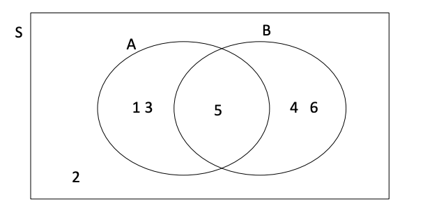
Example: experiment has the outcomes S={1, 2, 3, 4, 5, 6} where each outcome has an equal chance of occurring.
Let event A = {1, 3, 5} and event B = {4, 5, 6}.
Then A ∩ B = {5} and A U B = {1, 3, 4, 5, 6}. The Venn diagram is as follows:

Venn Diagram Example

Venn diagrams are useful to visualise the problem and help the understanding

Continuous sample space example

Measurements of the weight of a device are modelled with the sample space: S = {x | x > 0}, where S consists of positive real numbers
First set A1 = {x | 10 < x < 13},
Second set A2 = {x | 11 < x < 15}

Find union of A1 and A2, their intersection andcomplement of A1 and complement of A2.

Solution

• Union: A1 U A2 = {x | 10 < x < 15}
• Intersection: A1 ∩ A2 = {x | 11 < x < 13}
• Complement: A1’ = {x | 0 < x ≤ 10 or x ≥ 13}
• Complement: A2’ = {x | 0 < x ≤ 11 or x ≥ 15}

Probability

Random experiments have associated probability with them

To measure the probability, we assign a number between 0 and 1
    − 0 denotes probability that the event will not happen
    − 1 denotes probability that event will certainlyhappen

Example: If event has associated probability of 1/5, it will happen with 20% chance (1/5=0.2) and it will not happen with 80% chance (1-0.2=0.8)

Assigning probability- classical approach

If an event can occur in e different equally likely ways out of a total number of n possible ways, then the probability of the event is e/n.

Example: If coin is fair (head and tails are equally likely), probability of obtaining the tail is ½.

Example: If die is fair (all six outcomes are equally likely), probability of obtaining a three is 1/6.

Example: If there is one defective chip in 2000, the probability of picking it is 1/2000.

Assigning probability- frequencyapproach

For a very large number n, after n repetitions of an experiment, an event is observed to occur in e of these, then the probability of the event is e/n.
    − Also known as empirical probability of the event

Example: Coin is tossed 1,000 times and head occurred 493 times. Probability of a head is estimated as 493/1000=.493

Example: Die is tossed 1,000 times and number three is obtained 161 times. Probability of seeing a three is then 0.161

Probability axioms

If S is discrete sample space, all subsets correspond to events

Real number P(A) is associated with each event A in the space of events, C.
P is a probability function and P(A) is the probability of the event A, if the following axioms are satisfied:

Axiom 1: For each event A in space C, P(A)≥0

Axiom 2: For the sure event S in C, P(S)=1

Axiom 3: For mutually exclusive events A1, A2 12 ... in C, P(A1 U A2 U...) = P(A1)+P(A2)+...

Axiom 1 is about non-negativity ofprobability

Axiom 2 is about unitarity – there is an event, entire sample space, which will occur with probability of one

Axiom 3 is about additivity of mutually exclusive sets

Rest of facts about probabilities can be derived based on these axioms

The framework works with any assigned probabilities, as seen next

Probability Axioms: Simple Example

If we consider a single coin toss, then the coin will show either heads (H) or tails (T).
No assumption is made as to whether the coin is fair

Sample space S and space of event C are then: S={H,T} and C={Ø,{H},{T},{H,T}}

Probability of either head or tails is 1: P({H,T})=1
     • Sample space S is {H,T} and it is a sure event

Sum of probability of heads and probability of tails is one: P({H})+P({T})=1
     • This is true for both fair and biased coins

Probability of neither head nor tails is 0: P (Ø)=0

Assigning probabilities

Assigning probabilities provides a mathematical model

Coin or die examples: assigning equally likely probability to simple events is one way;
Frequency approach, where experiment is performed many times to measure probability empirically, is another

However, the success of the mathematical model must be tested by experiment just like other theories

Facts about probability

If A is a subset of B, then the probability of A is less than, or equal to the probability of B
    • Monotonicity property: If A is a subset of B, P(A)<P(B)
    • Example: Even die tosses are a subset of alltosses, (P(even)=1/2 and P(S)=1)

Probability is between zero and 1
Bounded values property: 1 ≥ P(A)≥0
    • Useful for checking calculations
        • If probability is outside of [0,1] interval, calculations are incorrect!

Probability of empty set is zero
    • Empty set property: P (Ø)=0

Complement probability: P(A’)=1-P(A)
    • Example: If probability that device will fail (A) is 0.05, then the probability that it will not fail (A’) is 0.95.
    • Example: If probability of obtaining a four in a die toss is 1/6, then the probability of not obtaining a four is 5/6.
    • Complement probability is used frequently to 17 simplify/check probability calculations

Facts: examples

If events A1, A2 , … and An are mutually exclusive and they form sample space S, then
   P(A1) + P(A2) + …+P(An)=1
    • Example: Probability of heads is ½ and probability of tails is ½. There are no other events: 1/2+1/2=1
    • Example: Probability that machine is working is 0.95. Probability that machine is not working is 0.05.

Probability of a Union

For any two events A and B, the probability of union is given by:
   P(A U B) = P(A) + P(B) - P(A ∩ B )

The reason probability of intersection is subtracted is that it is counted twice, in P(A) and P(B)

For mutually exclusive events, we get
    P(A U B) = P(A) + P(B)

P(A ∩ B )=0 because intersection is an empty set in this case

Probability of union vs sum of individual probabilities

Can probability of a union of two sets be larger than the sum of individual probabilities?

Formally, is it possible to have:
    P(A U B) > P(A) + P(B) ?

Answer:

Fact: P(A U B) = P(A) + P(B) - P(A ∩ B )
And P(A U B) > P(A) + P(B) would mean
P(A U B) = P(A) + P(B) - P(A ∩ B ) > P(A) + P(B)
0> P(A ∩ B ) which is impossible
Conclusion: P(A U B) > P(A) + P(B) is NOT possible

Example

A broken engine is randomly selected from a batch that is classified by faulty part A and faulty part B.
There are 1,000 broken engines, and 30 have faulty part A and 40 have faulty part B, while 20 have both faulty parts.
Find the probability that the engine has at least one faulty part.

Click here for Solution to the example  

Example: Solution

Then P(A) = 30/1000, P(B) = 40/100 and P(A ∩ B ) = 20/1000.

Therefore, P(A U B) = (30+40-20)/1000 = 50/1000