Lecture 7 – Random Variables

Random variable

Discrete probability distribution
– Probability mass function
– Properties: Unitarity and non-negativity

Cumulative distribution function

Expected Value (Mean) and Variance

Random Variables: Definition

Random variable: a variable which associates a number with the outcome of a random experiment
• In other words, random variable is a function which assigns a real number to each outcome in the sample space of a random experiment.

Random variable is typically denoted by uppercase letter such as X. However, the measured value of the random variable is denoted by a lowercase letter x.

For example, variable X denotes voltage and x = 10 Volts denotes specific measurement.

Example

A coin is tossed twice so the sample space is S = {HH, HT, TH, TT}.

Let X represent the number of heads that can come up. With each sample point we can associate a number for X:
Sample point: TT, TH, HT, HH
X :0, 1, 1, 2
Clearly, X is a random variable.

It is not the only random variable which can be defined on the sample space S

It is not the only random variable which can be defined on the sample space S: - Two to the power of number of heads - Sum of squares of number of heads and tails - Difference of number heads and tails (etc.)

Random variable which takes on a finite or countably infinite number of values is called a discrete random variable while one which takes on a noncountably infinite number of values is called a nondiscrete random variable.

Discrete Probability Distributions

Let X be a discrete random variable, and suppose that the possible values that it can assume are given by values x1, x2, x3, . . .
Suppose that these values are taken with probabilities given by P(X= xk) = f(xk ) for k =1, 2, . . .

It is convenient to introduce the probability mass function (pmf) f(x), also referred to as probability distribution, given by P(X = x) = f(x)

Key Properties of Discrete Probability Distribution

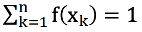
For a discrete random variable X with possible values x1, x2, …, xn, a probability mass function is a function such that non-negativity and unitary property hold:

Non-negativity property: f (xk )≥0 for all k=1,…,n

Unitary property:

There is a chance that a bit transmitted through a digital transmission channel is received in error.

Let random variable X denote the number of bits received in error in the next transmitted 2 bits.

The associated probability distribution of X isshown as follows: P(X=0)=.9; P(X=1)=.09; P(X=2)=.01;

Observe: probabilities are nonnegative and they add up to one (unitary property)

Find the probability of one or fewer bits in error.

Click here to view the solution

Cumulative Distribution Function

The cumulative distribution function (cdf) represents the probability that a random variable X, with a given probability distribution, will be found at a value which is less than or equal to x.

Mathematically, the definition of cdf is expressed as

F(x)=P(X ≤ x)= ∑xk≤ x f (xk)

Cumulative Distribution Function: Properties

CDF always takes values between 0 and 1 which can mathematically be expressed as: 0 ≤ F(x) ≤ 1

The above result is due to unitary property of pmf

CDF is non-decreasing function which can mathematically be expressed as: If x<y, then F(x)<F(y)

The above result is due to non-negativity property of pmf

Expected Value and Variance Of Random Variable

Mean or average value or expected value of random variable X with pmf f(x) is usually labelled μ or E[X]

It is symbolically written as: μ = E[X] = ∑k xkf(xk)

Variance of random variable X with pmf f(x) is usually labelled σ2 or Var[X] and is given mathematically as σ2 = Var[X] = ∑k (xk − μ)2f(xk)

Variance is always nonnegative number!

Expected Value Properties

• E[aX]=a E[X], for a constant a
• E[X+c]= E[X] +c, for some constant c
• E[X+Y]= E[X] + E[Y]
• If X and Y are independent: E[XY] = E[X] E[Y]

Variance Properties

Standard deviation is the square root of the variance: σ = sqrt( Var[X])

Var[aX] = a2 Var[X] for some constant a
σ2 = Var[X] = E[(X - μ)2]=E[X2 - μ2]=
= E[X2]- μ2=E[X2]-(E[X])2

Var[X+Y]=Var[X]+Var[Y] if X and Y are independent