Matlab on mobile phones!

Matlab for Android (free to use if you register with Mathworks – which is free)
https://play.google.com/store/apps/details?id=com.mathworks.matlabmobile&hl=en_GB

Matlab scripts for collecting sensor data from Android:
https://uk.mathworks.com/matlabcentral/fileexchange/47618-matlab-support-package-for-android-sensors

Matlab for iOS:
https://itunes.apple.com/gb/app/matlabmobile/id370976661?mt=8

Optional lab activity

Use mobile phone sensors to count number of steps
Android mobile phones:
https://uk.mathworks.com/examples/matlab/mw/mob ilesensor_product-mobilesensor_countingstepscounting-steps-by-capturing-acceleration-data-fromyour-android-8482-device

Apple iOS devices:
https://uk.mathworks.com/examples/matlab/mw/iossensor_product-iossensor_countingsteps-countingsteps-by-capturing-acceleration-data-from-your-apple174-ios-device

My research: various uses of probability in engineering

Paper about using randomness to improve positioning time of LED-based indoor positioning system which I have developed with my PhD student, Olaoluwa Popoola:
http://ieeexplore.ieee.org/document/8288588/
about my related research from the local newspaper, The Evening Times:
http://www.eveningtimes.co.uk/news/15287921.First_of_its_kind_tracking_ device_could_offer_fresh_hope_for_dementia_patients/#

Paper about using randomness to improve signals used in optical wireless communication. This is the work I have done with my former PhD student, Funmilayo Offiong and my colleague from Edinburgh, W.Popoola
http://ieeexplore.ieee.org/abstract/document/7922530/

Paper about using histogram comparison to spot anomalies in wireless data in order to fix broken telecommunications equipment. This work has been done with colleagues from the University of Edinburgh, including my former PhD student, Mostafa Afgani, and leading instrumentation company, Agilent.
https://www.hindawi.com/journals/ijdmb/2010/740594/abs/

Paper about using probabilities to help quantify load balancing in mobile communication with the aim of improving user throughput. This work is done with my colleagues at the University of Edinburgh, including Prof. Harald Haas and my former PhD student Ellina Foutekova:
http://ieeexplore.ieee.org/abstract/document/6389833/

More about my research:
http://researchonline.gcu.ac.uk/portal/en/persons/sinan- sinanovic(b9fa51d9-d950-41ac-9e18-d38ba88bbfae)/publications.html

Explore & Investigate

Learning by reading, by exploring and with your honours project

Lot of relevance for your current/future work

Find project topics that you feel passionate about

Go extra mile to push yourself

Previous students with strong project work landed good jobs

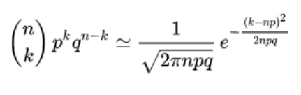
Video demonstration of binomial distribution

Practical demonstration of binomial distribution converging to Gaussian (normal) distribution
https://www.youtube.com/watch?v=4HpvBZnHOVI

Device is called Galton board or bean machine
When n is large, for k near np, we have:

Galton board

Sir Francis Galton was fascinated with the order of the bell curve that emerges from the apparent chaos of beads bouncing off of pegs in the Galton Board.
His quote: “Order in Apparent Chaos: I know of scarcely anything so apt to impress the imagination as the wonderful form of cosmic order expressed by the Law of Frequency of Error. The law would have been personified by the Greeks and deified, if they had known of it. It reigns with serenity and in complete self-effacement amidst the wildest confusion. The huger the mob, and the greater the apparent anarchy, the more perfect is its sway. It is the supreme law of Unreason. Whenever a large sample of chaotic elements are taken in hand and marshalled in the order of their magnitude, an unsuspected and most beautiful form of regularity proves to have been latent all along.” (Natural Inheritance (1889))

Lecture 10-11

Moving Average Filter

Outliers

Median

Median Filter

FFT, IDFT,

Zero Padding

Frequency Resolution

Linear Regression

Moving Average Filter

A moving average filter smooths data by replacing each data point with the average of the neighbouring data points defined within the span (or length) of the averaging window.

Averaging achieves smoothing by providing average value instead of sample value which potentially deviates significantly away from the mean

Example:
Apply the moving average filter of length three to the input sequence [x(1),
x(2), x(3) x(4)] and compute the second output.
x_smooth(2)=1/3*(x(1)+x(2)+x(3))
x_smooth(1)=x(1) (no smoothing)
x_smooth(3)=1/3*(x(2)+x(3)+x(4))
See Matlab smooth function:
https://uk.mathworks.com/help/curvefit/smoothing-data.html

Outliers

In the context of engineering data analysis, an outlier is an observation point that is distant from other observations. The outliers can occur due to - a) measurement errors, or - b) due to chance. Example: Summer temperatures in Glasgow in Celsius= [15 13 19 40 18] 40 is an outlier.

Averaging with outliers

A group of people (say 7 individuals) with no money and a billionaire are on average very wealthy but, clearly, average does not represent “typical” case.

Solution: use median!

Median is the middle value from the ordered list of values (in case of odd number of values) or average of the middle two, in case of even number of values

Median

Given a list of numbers, say 9, 1, 5, 3, 6, 7, 7, we first order the numbers: 1,3,5,6,7,7,9 and then pick the middle value, in this case 6. In case we have even number of values, say 4,2,7,1,8,9, we order them to get 1,2,4,7,8,9 and then pick average of the two middle values: (4+7)/2=5.5

Billionaire example: 0,0,0,0,0,0,0,10^9

Median is 0, while average is 1/8*10^9

Notice the huge difference between the median and the average

Average is much more sensitive to changes in individual values than the median

This fact is used to remove the “noise” (i.e. outliers)

For example, salt and pepper noise from images can be removed by applying median filter

Median Filter

A median filter runs through the signal entry by entry, replacing each entry with the median of neighbouring entries.
Example: x =[1, 40, 7, 3]. Assume that zeros are preceding and following the sequence.
Apply median filter to x.

Example:
x =[1, 40, 7, 3]. Assume that zeros are preceding and following the sequence. (mov. avg.)
x_median_filter(1)=median(0,1,40)=1 (1)
x_median_filter(2)=median(1,40,7)=7 (16)
x_median_filter(3)=median(40,7,3)=7 (16.7)
x_median_filter(4)=median(7,3,0)=3 (3)
At the end in (), moving average filter is shown – notice the huge difference in 2nd and 3rd outputs.
Moving average is sensitive to outliers, median filter is not.

Fast Fourier Transform (FFT)

The concept of Fast Fourier Transform

Fast Fourier transform (FFT) is an algorithm which takes samples of a signal over a period of time and converts them into frequency components. These components are single sinusoidal oscillations at distinct frequencies, each with their own amplitude and phase.

FFT is computed the fastest when applied over a signal which has exact power of two number of samples (due to nature of FFT algorithm)

Difference between FFT and Discrete Fourier Transform (DFT)

Discrete Fourier Transform (DFT) is computed in a fast and efficient manner by the Fast Fourier Transform (FFT).
In particular, DFT requires on the order of N^2 operations, while FFT requires on the order N*log(N) operations.

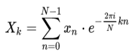
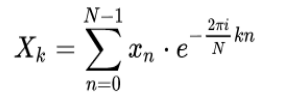
Discrete Fourier Transform: DFT:

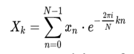
where n and k go from 0 to N-1

Inverse Discrete Fourier Transform

• Inverse Discrete Fourier Transform

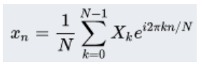
Compare with Discrete Fourier Transform

DFT computation example

We have: x=(1, 2-i, -i, -1+2i).
Therefore N=4. Also, indices of x go from 0 to 3.
Using

we have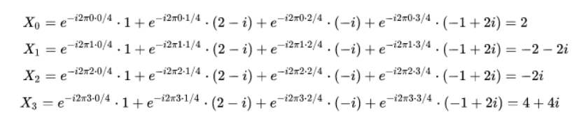

X = (2, -2-2i, -2i, 4+4i)
Check using IDFT!
In Matlab, use fft

Zero padding

In the context of FFT, zero-padding adds zeros to the time domain signal. Two benefits of zero padding:
• One: signal can have length of the exact power of two which speeds up FFT.
• Two: zero-padding can help better reveal frequency content, although it does not increase spectral resolution.

Improving frequency resolution

In order to improve frequency resolution, time domain signal should be observed for longer before FFT is computed.

Linear regression

Aim is to minimise sum of square distances from the line y=a+bx to n points (xi yi)
• Such line is the best linear square fit
• We find a and b as follows: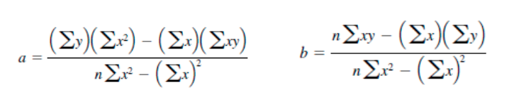

In Matlab, we have seen using polyfit command to compute best linear (and parabolic) fits