Recursion

In computer programming, recursion is concerened with the ability of a function (or subroutine) to call itself.

Factorial Function

On of the best known recursive functions is the factorial function. This is defined as:

$n! = (n)(n-1)(n-2)...(2)(1)$

$ = (n)(n-1)!$

also $(n-1)! = (n - 1)(n - 2)!$ and so on

Example

$3! = (3)(2)(1) = 6$

$4! = (4)(3!) = (4)(6) = 24$

$5! = (5)(4!) = (5)(24) = 120$

Now as the factorial function is a function we have values for $0!$ and $1!$.

$0! = 1$

$1! = 1$

The factorial function is a special case of the gamma function where $T(n) - nT(n-1)$.

Programming a Factorial Function

We might have an intial attempt at writing code as follows:

declare function factorial $(int n)$

return $n \times$ factorial $(n -1)$

If this psuedo code is tested, then we would have for example for $n = 3$:

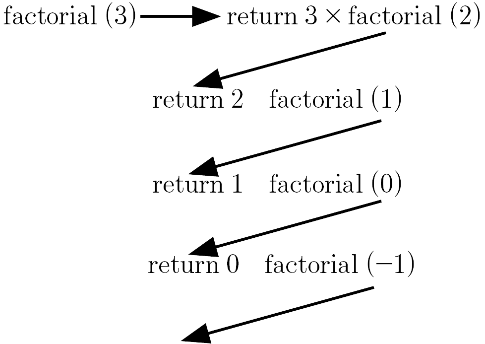
Clearly, there is a problem, as there is no end to the call of the function, the computer would eventually run out of stack space and crash

We need a halting case ( or base case ) and we need to deal with incorrect input.

The $n$ in the factorial function should not be less than $0$. If it is, an error value can be returned. Also 0! = 1 and 1! = 1.

So psuedo code could look like:

declare function factorial $(int\; n)$

if $n < 0$ the return $0$ // error code

else if $n = 0$ or $n = 1$ return $1$

else return $n \times$ factorial $(n - 1)$

Now if we look at some examples

factorial $(-4) = 0$; return $0$, so it is an error

factorial $(0) = 1$

factorial $(1) = 1$

factorial $(4) = (4)(3)(2)(1) = 24$

A Recursive Power Function

Computes an integer power of a floating point number

double power(double base, int exponent) {
    if (exponent < 1) {
        return 1.0;
    } else {
        return power(base, exponent-1) * base;
    }
}

The function is called as follows:

System.out.println( power(1.7, 3) );

Initial bindings

base = 1.7

exponent = 3

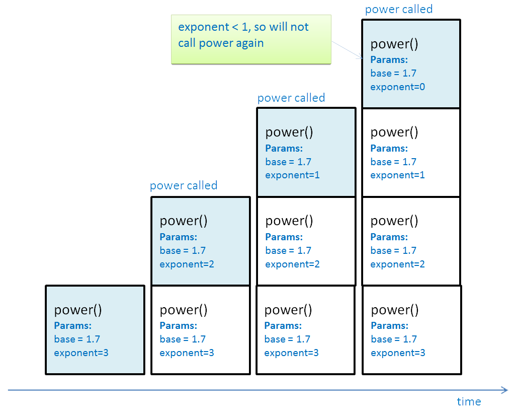
This diagram shows how the contents of the call stack change as recursive calls are made. Each time power executes, it makes another call to power, and pushes a new stack frame to the call stack. The value of the exponent parameter is different each time – look at the code to see why. At the fourth call, exponent is now < 1, so the other branch of the if statement executes and power is not called again. This is the stopping condition – without it the recursion would go on forever!

Call stack with recursive calls

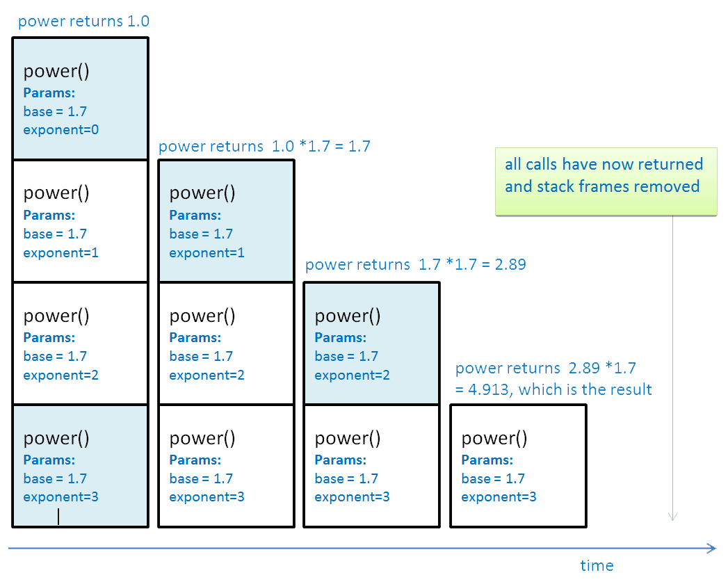
In the fourth call, power returns 1.0 and that frame is popped from the stack. Execution returns to the third call, which returns the result of calculating:

power(base, exponent-1) * base

which is:

value returned by fourth call * base
= 1.0 * 1.7
= 1.7

Now the third frame is popped from the stack and execution returns to the second call, which in turn returns the result of calculating:

value returned by third call * base
= 1.7 * 1.7
= 2.89

Now the second frame is popped from the stack and execution returns to the first call, which in turn returns the result of calculating:

value returned by second call * base
= 2.89 * 1.7
= 4.913

Each return does the following:

Pops a frame off of the stack

Restores its data state

Replaces the call to power with the return value

Continues execution at the return address

Call stack as recursive calls return

Recursion and RAM

Recursive functions may require more space in memory than non-recursive calls. With some deeply recursive algorithms this can be a problem. It is possible to run out of memory space on the stack – stack overflow.

It can also be a problem with poorly written recursive functions with bad stopping condition definitions (result is like an infinite loop only on the stack)

Advantages of recursion

Recursion’s big advantage is the elegance with which it embodies the solution to many problems

It closely follows the mathematical definition of many functions

This makes it easier to prove correctness

Some problems are much easier to solve recursively than iteratively, e.g. Towers of Hanoi

Disadvantages of recursion

Use of system resources slows the process down compared to iterative solutions, although this may not be a big factor on modern machines

Possibility of stack overflow

Difficult to ‘think recursively’

Fibonacci Numbers

The Fibonacci number are also recursive.

The numbers start as follows:

$1, 1, 2, 3, 5, 8, 13, \cdots$

Now the first number $f_1 = 1$, the second number $f_2 = 1$.

The third number is formed as follows:

$f_3 = f_2 + f_1 = 1 + 1 = 2$

The fourth number is:

$f_4 = f_3 + f_2 = 2 + 1 = 3$

In general,

$f_n = f_{n-1} + f_{n-2}$

Strangely though, these numbers appear in computing and in biology in a natrual way.

Merge Sort

The sorting process is used to arrange the items in a collection, for example an array, in an increasing or decreasing order. Sorting algorithms would be covered in Week 6 and 7 but here we study Merge sort, a very efficient sorting algorithm that is based on divide-and-conquer technique nicely implemented using recursion.

Merge sort has a time complexity of Ο(n log n).

Merge sort has two steps, divide and merge:

1) The array is divided into equal halves and this halving process is performed recursively until an array of size one results; an only item in an array is already sorted.

2) The merging step is then performed that combines two array halves (that have already been sorted) into one larger array, ultimately combining the whole array by merging (and thus sorting the original array).

This merge sort algorithm can be expressed as,

Divide the array in two halves

Merge sort the first half

Merge sort the second half

Merge the two halves

Psuedocode

mergeSort ( array arr of size n )
{
       if ( n == 1 ) return arr 
       left_arr = arr[0] to arr[n/2]
       right_arr = arr[n/2+1] to arr[n]
       left_arr = mergeSort( left_arr )
       right_arr = mergeSort( right_arr )
       return merge( left_arr, right_arr )
}

merge(leftarr as array, rightarr as array)
{
resultarr as array
    	
while ( length(leftarr) > 0 and length(rightarr) > 0)

        if(smallest item in leftarr < smallest item in rightarr)
            add (smallest item in leftarr) to resultarr
            remove (smallest item from leftarr)
        else
            add (smallest item in rightarr) to resultarr
            remove (smallest item from rightarr)
 
    	if length(leftarr) > 0
        add leftarr to resultarr
    	if length(rightarr) > 0
        add rightarr to resultarr
    
return resultarr
}

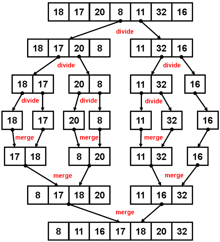
Recursive Calls in Merge Sort

The array is recursively divided into two halves until both halves consist of only a single item, which can be considered sorted. At this point, the merge is performed that puts the items from both halves in a sorted order. This merge process is repeated until whole of the array is sorted.

Summary

Recursion is a problem-solving technique where a method calls itself again and again on progressively smaller version of the original problem.

A recursive solution must have a terminating or base case at which point no further method calls are made.

Recursion can result in very simple and elegant solutions.

Recursive solutions are slower and require more memory compared to iterative solutions due to maintaining the call stack.

Merge sort is an efficient sorting algorithm which uses a divide-and-conquer strategy.