Broadly, there are 4 types of Machine Learning algorithms:

Supervised machine learning

Unsupervised machine learning

Semi-supervised machine learning

Reinforcement machine learning

Supervised machine learning

Supervised machine learning is where you have input variables ($X$) and an output variable ($Y$) – labelled data - and you use an algorithm to learn the mapping function from the input to the output.

$$Y = f(X)$$

The goal is to approximate the mapping function so well that when you have new input data ($x$) that you can predict the output variables ($y$) for that data.

It is called supervised learning because the process of an algorithm learning from the training dataset can be thought of as a teacher supervising the learning process. We know the correct answers, the algorithm iteratively makes predictions on the training data and is corrected by the teacher. Learning stops when the algorithm achieves an acceptable level of performance.

The majority of practical machine learning uses supervised learning.

Supervised learning problems can be further grouped into regression and classification problems:

Classification: A classification problem is when the output variable is a category, such as “red” or “blue”, or “disease” and “no disease”.

Regression: A regression problem is when the output variable is a real value, such as “dollars” or “weight”.

Some popular examples of supervised machine learning algorithms are:

Linear regression for regression problems

Random forest for classification and regression problems

Support vector machines for classification problems

Unsupervised machine learning

Unsupervised learning is where you only have input data (X) and no corresponding output variables – unlabelled data.

The goal for unsupervised learning is to model the underlying structure or distribution in the data in order to learn more about the data. These are called unsupervised learning because unlike supervised learning above there is no correct answers and there is no teacher. Algorithms are left to their own devises to discover and present the interesting structure in the data.

Unsupervised learning problems can be further grouped into clustering and association problems:

Clustering: A clustering problem is where you want to discover the inherent groupings in the data, such as grouping customers by purchasing behavior.

Association: An association rule learning problem is where you want to discover rules that describe large portions of your data, such as people that buy $X$ also tend to buy $Y$.

Some popular examples of unsupervised learning algorithms are:

k-means for clustering problems

Apriori algorithm for association rule learning problems

Semi-supervised machine learning

Problems where you have a large amount of input data ($X$) and only some of the data is labelled ($Y$) are called semi-supervised learning problems. This type of problem falls somewhere in between supervised and unsupervised learning.

To deal with this type of problem, both labelled and unlabelled data can be used for training: You can use unsupervised learning techniques to discover and learn the structure in the input variables. You can also use supervised learning techniques to make best guess predictions for the unlabelled data, feed that data back into the supervised learning algorithm as training data and use the model to make predictions on new unseen data.

Many real world machine learning problems fall into this area. Because it can be expensive or time-consuming to label data as it may require access to domain experts. Whereas unlabelled data is cheap and easy to collect and store.

A good example is a photo archive where only some of the images are labelled, (e.g. dog, cat, person) and the majority are unlabelled.

Reinforcement machine learning

Reinforcement machine learning is a learning method that interacts with its environment by producing actions and discovers errors or rewards. Trial and error search and delayed reward are the most relevant characteristics of reinforcement learning. This method allows machines and software agents to automatically determine the ideal behaviour within a specific context in order to maximize its performance. Simple reward feedback is required for the agent to learn which action is best; this is known as the reinforcement signal.

Linear regression is a linear approach to modelling the relationship between a scalar response variable $y$ (also called outcome or dependent variable) and one or more explanatory variables $X$, (also called predictors, independent variables).

Simple linear regression concerns the study of only one predictor variable. Multiple linear regression concerns the study of two or more predictor variables.

Simple linear regression

In simple linear regression, we predict scores on one variable from the scores on a second variable. The variable we are predicting is referred to as $Y$. The variable we are basing our predictions on is referred to as $X$. In simple linear regression, the predictions of $Y$ when plotted as a function of $X$ form a straight line.

The example data in Table below are plotted in the Figure next to it. You can see that there is a positive relationship between $X$ and $Y$. If you were going to predict $Y$ from $X$, the higher the value of $X$, the higher your prediction of $Y$.

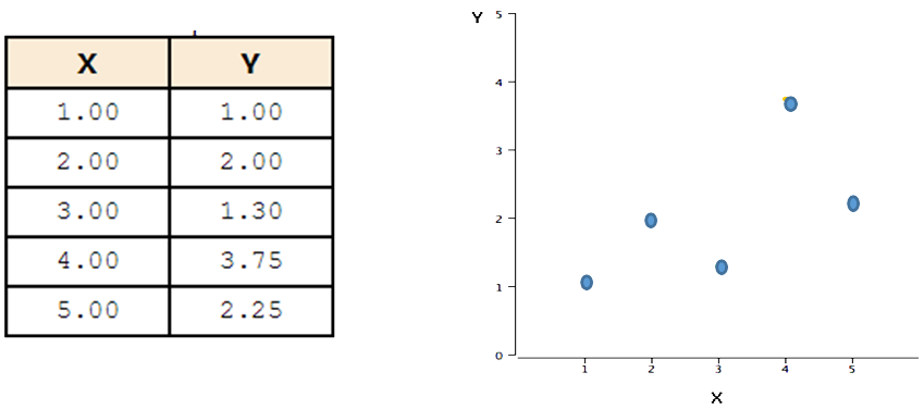
Linear regression aims to finding the best-fitting straight line through the points. The best-fitting line is called a regression line.

The black line in the figure below is the regression line and consists of the predicted score $Y$’ for each possible value of $X$. The vertical lines from the points to the regression line represent the errors of prediction (the difference between the predicted $Y$’ and the observed $Y$, i.e., $Y-Y$’). As you can see, when $x=1$, its error of prediction is small (i.e., $-0.21$ as listed in the table below). By contrast, when $x=4$, its error of prediction is big (i.e., $1.265$ as listed in the table below).

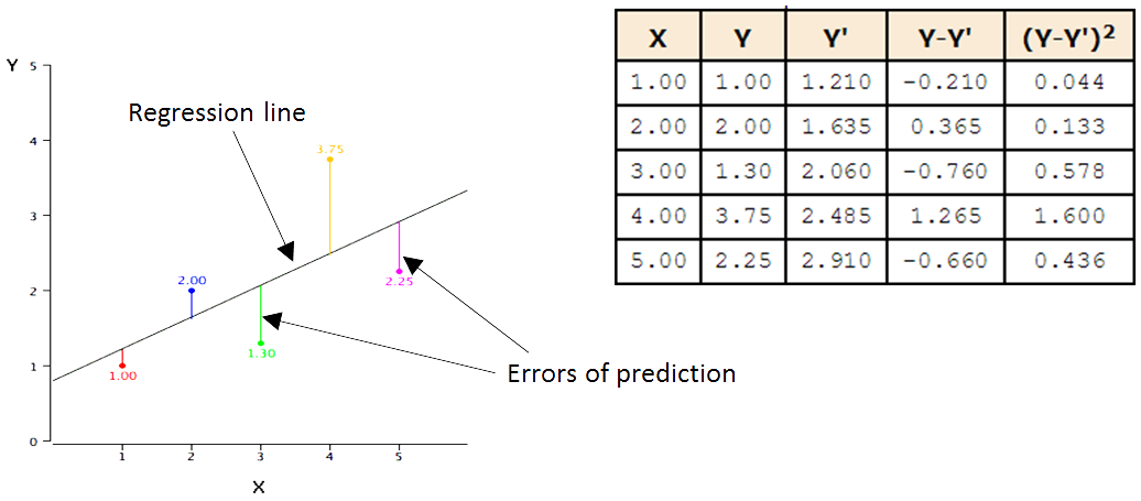
There are various Criteria on what is meant by “best-fitting line”. Among them, least squares criterion is most commonly-used, which specifies the line that minimizes the sum of the squared errors of prediction as the best-fitting line, i.e., regression line.

Computing the Regression Line

Let us use $y_i$ denotes the observed response for experimental unit i

$x_i$ denotes the predictor value for experimental unit $i$

$\tilde{y}_i$ is the predicted response (or fitted value) for experimental unit $i$

Then, the equation for the best fitting line can be represented as:

$$\tilde{y}_1 = b_0 + b_1x_i$$

The prediction error is:

$$e_i = y_i - \tilde{y}_i$$

The least squares criterion aims to find the vales of $b_0$ and $b_1$ that minimize:

$$Q = \sum_{i=1}^{n} (y_i - \hat{y}_i)^2$$

Take the derivative with respect to $b_0$ and $b_1$, set to $0$, and solve for $b_0$ and $b_1$, the "least squares estimates" for $b_0$ and $b_1$ are:

$$b_0 = \tilde{y} - b_1\tilde{x}$$

$$b_i = \frac{\sum_{i=1}^{n} (x_i - \tilde{x})(y_i - \tilde{y})}{\sum_{i=1}^{n} (x_i - \tilde{x})^2}$$

Using these formula to calculate the $b_0$ and $b_1$ in the regression line for the example data above, we have:

$b_0 = 0.785$
$b_1 = 0.425$

And the equation for the regression line is:

$$y = 0.785 + 0.425x$$

Multiple Linear Regression

The model of Multiple Linear Regression is:

$$y_i = \beta_0 + \beta_1x_i,_1 + \beta_2x_i,_2 + \cdots + \beta_{p-1}x_i,_{p-1} + \in_i.$$

We assume that the $\in_i$ have a normal distribution with mean $0$ and constant variance $\sigma^2$. These are the same assumptions that we used in simple regression with one $x$-variable.

The word "linear" in "multiple linear regression" refers to the fact that the model is linear in the parameters. The estimates of the $\beta$ coefficients are the values that minimize the sum of squared errors for the sample.

SVM (Support Vector Machine) is a supervised machine learning algorithm which can be used for both classification or regression challenges, while more widely be used in classification problem.

The objective of the SVM algorithm is to find a hyperplane in an N-dimensional space (N is the number of features used in the algorithm) that distinctly classifies the data points.

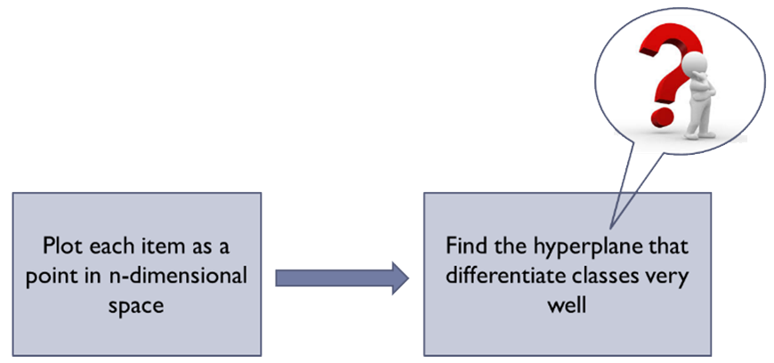
Hyperplanes are decision boundaries that help classify the data points. Data points falling on either side of the hyperplane can be assigned to different classes. A hyperplane is a generalization of a plane. In one dimension, a hyperplane is called a point; in two dimensions, it is a line; in three dimensions, it is a plane; in more dimensions you can call it a hyperplane.

Some examples

Let us start from 2D.

Example one - accuracy

In the figure below, we have three hyperplanes (A, B and C), which one is the right hyperplane to classify star and circle?

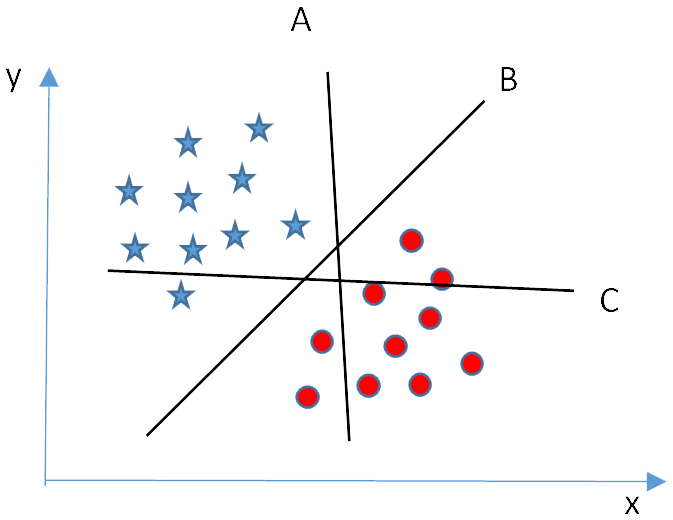
As mentioned earlier, a hyperplane is used to separate points into different classes. In the figure above, hyperplane ‘B’ has the best performance for this job.

Example two - margin

Now, we have another three hyperplanes (B1, B2 and B3) and all separate the points into different classes correctly. Which one is the right hyperplane?

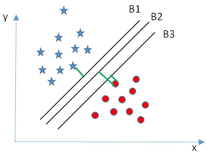
In this case, we select the hyperplane has the maximum distance with the nearest point in the dataset. i.e., hyperplane B2 is the right one for this dataset. Double of the distance between a hyperplane and the nearest point is called as Margin. The goal of a SVM is to find the optimal separating hyperplane which maximizes the margin of the training data.

Example three – accuracy vs. margin

In the figure below, which hyperplane is the right one?

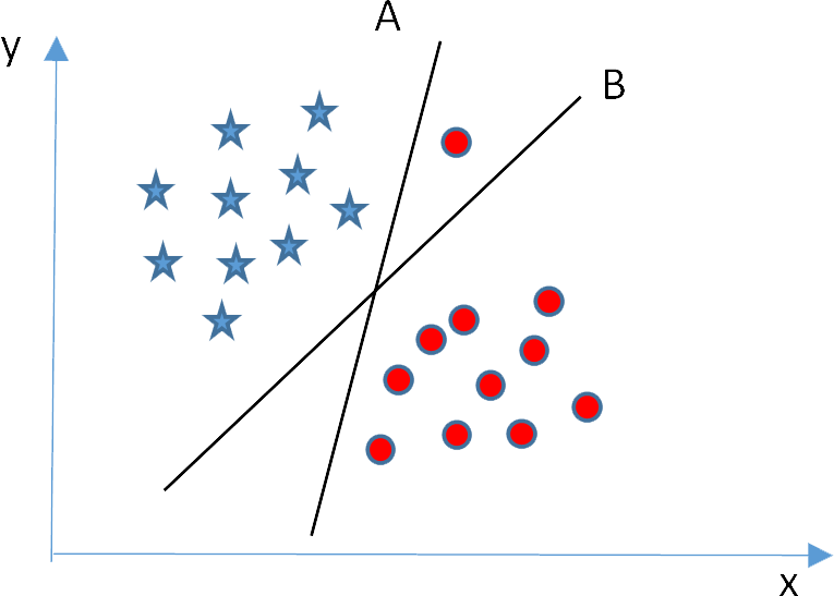
If we use the margin criterion, it looks like hyperplane B has bigger margin compared to hyperplane A. But, in SVM, accuracy has higher priority than maximizing margin. In this example, hyperplane B has a classification error, and hyperplane A classified all points corrctly. Therefore, hyperplane A is the right one.

Example four – outlier

In the following figure, it is impossible to separate the stars and circles with a straight line, as there is a circle lies in the territory of the stars. As mentioned in week 6, this circle is like an outlier of the circle class. SVM is able to ignore outlier and find the hyperplane with maximum margin, i.e., hyperplane B for this example.

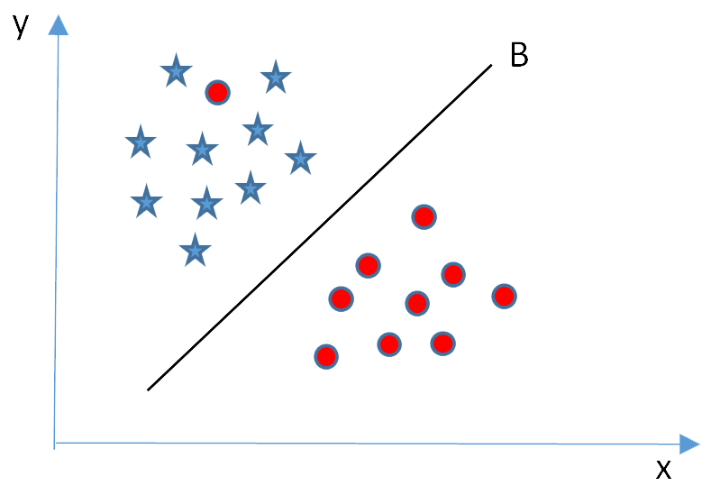
Example five – Kernel

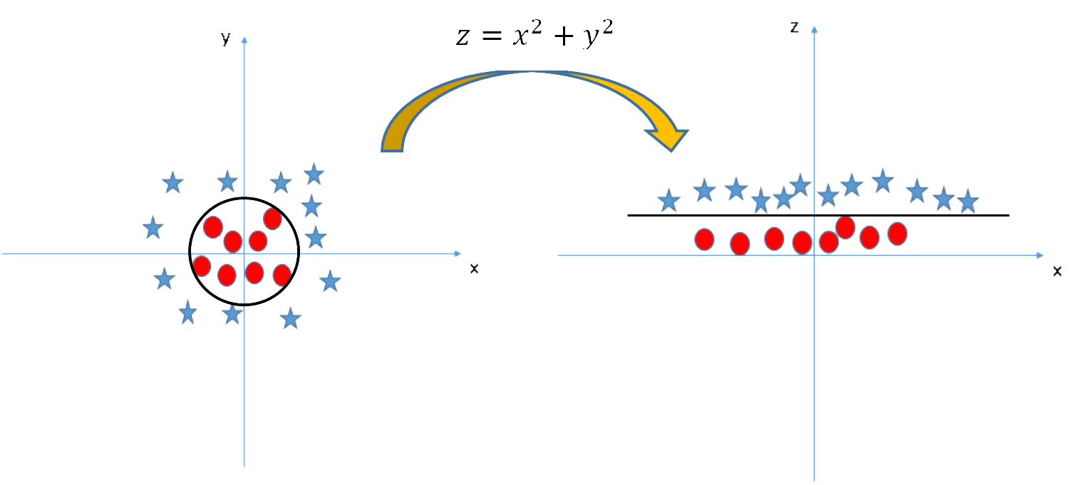
In the scenario below, the stars and circles in the left figure cannot be segregated with a linear hyperplane. SVM can solve this problem by introducing an additional feature $z=x^2+y^2$. As illustrated in the right figure, it is easy to have a linear hyperplane between the star and circle classes now. This additional feature has been added via the Kernel technique in SVM. SVM use kernels to concert not separable problem to separable problem, which is mostly useful in non-linear problem

Equation of a hyperplane

An equation of a line is:

$$y = ab + b$$

The equation of a hyperplane is an inner/dot/scalar product of two vector:

$$W^TX = 0$$

in 2D

$$W = \pmatrix{-b \\ -a \\ \;1}, X = \pmatrix{1 \\ x \\ y}, \;\text{and}\; W^TX = y - ax - b$$

It is easier to work in more than two dimensions with this notation. the vector $W$ will always be normal to the hyperplane.

Or, a hyperplane can also be represented as:

$$WX + b = 0$$

where,

$$ W = \pmatrix{-a \\ \;\;1}^T, \;\; X = \pmatrix{x \\ y}, \;\text{and}, \; WX + b = y - ax + b$$

Finding the optimal hyperplane

As mentioned above, finding the optimal hyperplane is to find the hyperplane with the biggest margin.

Then, how can we find the biggest margin? This problem can be defined as: Given a dataset $D$

$$D = \{(x_i, y_i) \mid x_i \in \mathbb{R}^P, y_i \in \{-1, 1\}\}_{i=1}^{n} $$

select two hyperplanes which separate the data with no points between them and maximize their distance (the margin).

Now, let us see how to find the maximum distance (the margin).

Assuming there is a hyperplane $H$ separating the dataset $D$ and satisfying:

$$WX + b = 0$$

Select two other a hyperplane $H_1$ and $H_0$:

$$WX + b = \delta \\ WX + b = -\delta$$

In order to simplify the problem, we can set $\delta=1$, so hyperplane $H_1$ and $H_0$ are:

$$WX + b = 1 \\ WX + b = -1 $$

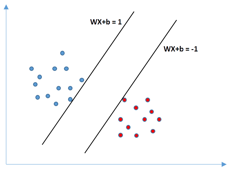
To be sure there is no pints between then:

For each vector $X_i$, either:

$WX_i+b≥1$ for $X_i$ having the class $1$ , i.e., $y_i=1$;

Or $WX_i+b≤-1$ for $X_i$ having the class $-1$, i.e., $y_i=-1$

These two constraints can be combined into a unique:

$y_i (WX_i+b)≥1$ for all $1≤i≤n$

Next, we calculate the distance between the two hyperplanes:

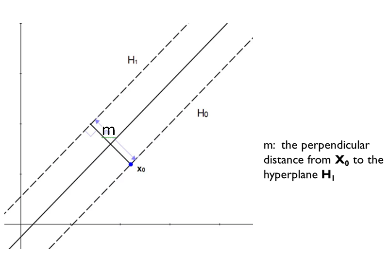
As illustrated in the figure above, the distance m is the perpendicular distance from a point on the hyperplane $H_0$, e.g., point $X_0$, to the hyperplane $H_1$, define a vector $K$, which is perpendicular to $H_1$ and has the length of m. Moving the start point of vector $K$ to point $X_0$, the end point of vector $K$, i.e., point $Z_0$, will be on hyperplane $H_1$ , so:

$WZ_0+b=1$

$as Z_0=X_0+K , \;\text{then}:$

$W \cdot(X_0+K)+b=1$

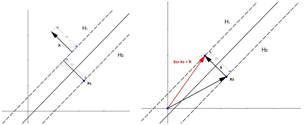
Vector $W$ and $K$ have the same direction, so vector $K$ can be written as $m \frac{W}{\|W\|}$ , put it in the formula above, we have:

$W \cdot(X_0+m \frac{W}{\|W\|} )+b=1 \\ \\ W \cdot X_0+m \frac{W \cdot W}{\|W\|} +b=1 \\ \\ W \cdot X_0+m \frac{\|W\|^2}{\|W\|} +b=1 \\ \\ W \cdot X_0+m\|W\|+b=1 \\ \\ W \cdot X_0+b=1-m\|W\|$

as $X_0$ is on $H_0$, then $W \cdot X_0+b=-1$, so:

$-1=1-m\|W\|$

$m\|W\|=2$

$m=\frac{2}{\|W\|}$

Finally, we find out that maximizing the margin is the same as minimizing the norm of W. this give us the following optimization problem:

Minimize $\|W\|$ in $(W,b)$,

subject to

$y_i (WX_i+b)≥1$ for all $1≤i≤n$

Solve this problem, then we will have the equation for the optimal hyperplane!

Pros and Cons

SVM has many advantages, which include:

It works really well with clear margin of separation

It is effective in high dimensional spaces.

It is effective in cases where number of dimensions is greater than the number of samples.

It uses a subset of training points in the decision function (called support vectors), so it is also memory efficient.

Also, SVM has limitations such as:

It doesn’t perform well, when we have large data set because the required training time is higher

It also doesn’t perform very well, when the data set has more noise i.e. target classes are overlapping

SVM doesn’t directly provide probability estimates, these are calculated using an expensive five-fold cross-validation.