-
Artificial Neural Network – Architecture and activation function
Artificial neural networks (ANN) are one of the main tools used in machine learning. As the “neural” part of their name suggests, they are vaguely inspired by the biological neural networks that constitute human brains.
Human brain is one of the wonders of the world. Consider the following handwritten digits:
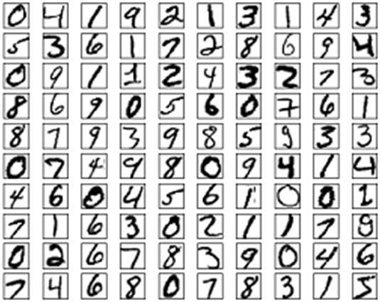
It is effortless for human to recognize those digitals. While it is difficult if you attempt to write a computer program to recognize digits like those above. What seems easy when we do it ourselves suddenly becomes extremely difficult. For example, if you create an algorithm to simulate how we recognize shapes "a 9 has a loop at the top, and a vertical stroke in the bottom right", it turns out to be not so simple. When you try to make such rules precise, you quickly get lost in a morass of exceptions and caveats and special cases!
Artificial neural networks approach the problem in a different way: it learns from a large number of examples, known as training examples.
Human neurones

In the human brain, a typical neuron collects signals from others through a host of dendrites. The neuron sends out spikes of electrical activity through an axon, which splits into thousands of branches. At the end of each branch, a structure called a synapse converts the activity from the axon into electrical effects that inhibit or excite activity from the axon into electrical effects that inhibit or excite activity in the connected neurones.
When a neuron receives excitatory input that is sufficiently large compared with its inhibitory input, it sends a spike of electrical activity down its axon. Learning occurs by changing the effectiveness of the synapses so that the influence of one neuron on another changes.
Perceptrons
The term ‘oerceptron’ was coined by Frank Rosenblatt in the 60’s. Perceptrons are single-layer ANN. Perceptrons mimic the basic idea behind the mammalian visual system.
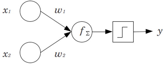
In the example shown above, the perceptron has two inputs $x_1$ and $x_2$.
A perceptron can weigh up different kinds of evidence in order to make decisions. By varying the weights and the threshold, we can get different models of decision making.
Let us write $\sum_j w_j x_j$ as a dot product:
$w \cdot x \equiv \sum_j w_jx_j$
Where $w$ and $x$ are vectors with components of the weights and inputs separately.
Also, we can move the threshold to the other side fo the inequality and replace it by:
$b= -$ threshold
$b$ is known as perceptron’s bias.
Then, the output of perceptron can be rewritten as:

The bias is a measure of how easy it is to get the perceptron to fire (output =1).
Perceptrons can be used is to compute the elementary logical functions which underlying computation, functions such as AND, OR, and NAND. For example, suppose we have a perceptron as below:
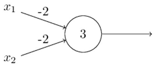
A NAND gate $x_1$ $x_2$ Output $ w \cdot x + b = (-2) * x_1 + (-2) * x_2 + 3$ $x_1$ NAND $x_2$ 0 0 1 1 0 1 1 1 1 0 1 1 1 1 0 0 Because NAND gates are universal for computation, it follows that perceptrons are also universal for computation. we can use networks of perceptrons to compute any logical function.
As a learning algorithm, it would be preferring to see that a small change in some weight (or bias) in the network will cause only a small corresponding change in the output from the network. However, this is not what happens in a perceptron network. In fact, a small change in the weights or bias of any single perceptron in a network can sometimes cause the output of that perceptron to completely flip, say from 0 to 1. To overcome this problem, a new type of artificial neuron called Sigmoid Neurons is introduced.
Sigmoid neurons
Sigmoid neurons are similar to perceptrons (as illustrated below). Just like a perceptron, a sigmoid neuron has inputs $x_1, x_2, …, x_n$, but instead of just take $0$ or $1$, inputs of a sigmoid neuron can be any value between $0$ and $1$.
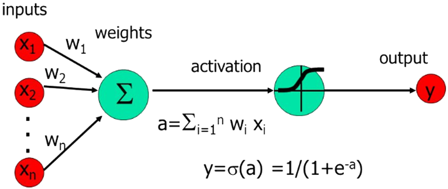
The sigmoid neuron also has weights for each input and overall bias. But the output of sigmoid neuron is not $0$ or $1$. Instead, it is:
$$\sigma (w \cdot x + b)$$
where $\sigma$ is called the sigmoid function, and is defined by:
$$\sigma (z) \equiv \frac{1}{1 + e ^{-z}}.$$
So, the output of a sigmoid neuron is:
$$\frac{1}{1 + exp(-\sum_j w_jx_j - b)}$$
The shape of a sigmoid function $\sigma$ is shown below. As you can see, the shape of a sigmoid function is a smoothed out version of a step function. The smoothness of $\sigma$ means that small changes in the weights and bias will produce a small change in the output. It is true there are smoothed functions, while using $\sigma$ will simplify the algebra: exponentials have lovely properties when differentiated.

The architecture of Neural Networks
In a neural network, e.g., the one shown below, the leftmost layer is called the input layer, and the neurons within the layer are called input neurons. The rightmost or output layer contains the output neurons, or, as in this case, a single output neuron. The middle layer is called a hidden layer, since the neurons in this layer are neither inputs nor outputs. In this example, there are two hidden layers. Historically, such multiple layer networks are sometimes called multilayer perceptrons or MLPs, despite being made up of sigmoid neurons, not perceptrons.
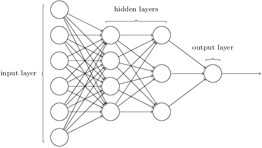
The design of the input and output layers of a neural network is often straightforward. The number of neurons in the input layer equals to the number of input variables. The number of neurons in the output layer direct depends on the number of possible output values. However, there can be quite an art to the design of the hidden layers. There are no simple rules of thumb for the design of hidden layers.
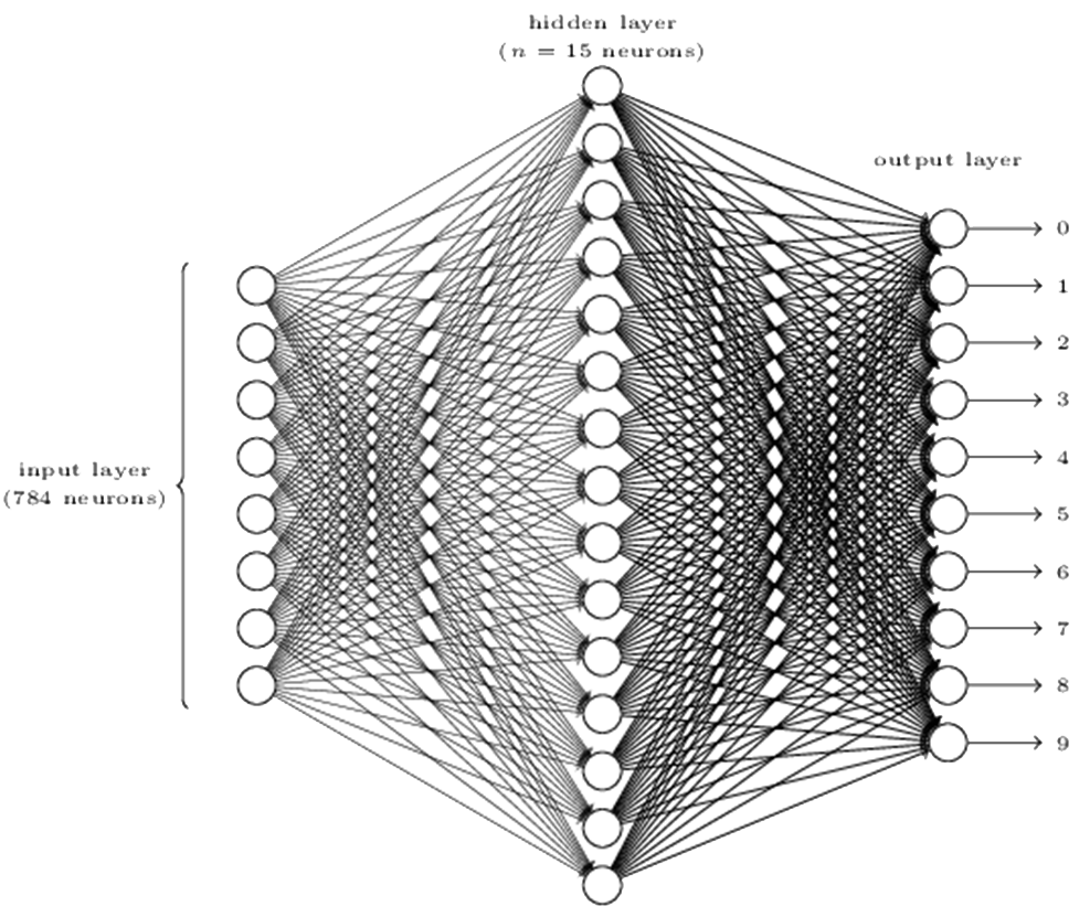
Taking the handwritten image determination as an example, if the image is a 28 by 28 greyscale Image, we can have 28*28=784 input neuron, with each of the neurons represent a pixel’s intensity. The output layer can have 10 output neuron, with each of them indicate a digit. If we use one hidden layer with 15 neurons, the structure of the neural network for handwritten image determination will be:
Feedforward or feedback
There are two major types of ANN: feedforward neural networks and feedback neural networks.
In feedforward NNs, signals travel from input to output. There are no loops in the network. Information is always fed forward, never fed back. Feedforward NNs are extensively used in pattern recognition.
In feedback NNs, data can flow in multiple directions. These models are also called Recurrent neural network. Recurrent neural networks are much closer in spirit to how human brains work than feedforward networks. Recurrent neural nets had been less influential than feedforward networks, in part because the learning algorithms for recurrent nets were less powerful.
-
Artificial Neural Network – learning algorithm
Artificial neural networks find solution to problems by learning from a large number of examples. The procedure used to carry out the learning process in a neural network is called the training algorithm. The learning problem in neural networks is formulated in terms of the minimization of a cost function.
Quadratic Cost function (MSE - Mean Squared Error)
The Quadratic Cost function $C$, also known as the Mean Square Error (MSE), is defined as:
$$C(w,b) \equiv \frac{1}{2n} \sum_x \| y(x) - a \|^2 $$
Where $w$ denotes the collection of all weights in the neural network, $b$ represents all the biases, $n$ is the total number of training inputs, $a$ is the vector of outputs from the network when $x$ is input, and the sum is over all training inputs, $x$ .
Using a smooth cost function like the quadratic cost it turns out to be easy to figure out how to make small changes in the weights and biases so as to get an improvement in the cost.
The aim of training algorithm is to minimize the cost $C(w,b)$ as a function of the weights and biases, i.e., to find a set of weights and biases which make the cost as small as possible. Commonly, the algorithm known as gradient descent is used to do that.
Learning with gradient descent
Assuming $C$ is a function of two variables $v_1$ and $v_2$, as illustrated in the figure below, and we want to find where $C$ achieve its global minimum.
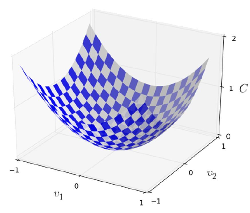
let's think about what happens when we move a small amount $\Delta v_1$ in the direction $v_1$, and a small amount $\Delta v_{21}$ in the direction $v_2$. Calculus tells us that $C$ changes as follows:
$$\Delta C \approx \frac{\partial C}{\partial v_1} \Delta v_1 + \frac{\partial C}{\partial v_2} \Delta v_2.$$
If we can find a way of choosing $\Delta v_1$ and $\Delta v_2$ so as to make $\Delta C$ negative, we should be able to find where $C$ achieve its global minimum.
Define $\Delta v$ to be the vector of changes. In 2D, it is:
$$\Delta v \equiv (\Delta v_1, \Delta v_2)^T $$
Where $T$ is the transpose operation.
Also, define the gradient of $C$ to be the vector of partial derivatives:
$$\nabla C \equiv \Big(\frac{\partial C}{\partial v_1}, \frac{\partial C}{\partial v_2}\Big)^T $$
Then, $\Delta C$ can be rewritten in terms of $\Delta v$ and $\nabla C$:
$$\Delta C \approx \nabla C \cdot \Delta v $$
If we choose:
$\Delta v = \eta \nabla C$(a)
Where $\eta$ is a small, positive parameter (known as the learning rate)
Then:
$$\Delta C \approx - \eta \nabla C \cdot \nabla C = - \eta \| \nabla C \|^2 $$
Because $\| \Delta C\|^2 \ge 0$, this guarantees that $\Delta C \le 0$, i.e., $C$ will always decrease, never increase, if we change $v$ according to the prescription above. So we will use equation (a) to compute a value for $\Delta v$, then the new value of $v$ is:
$$v \to v^{'} = v - \eta \nabla C $$
To make gradient descent work correctly, we need to choose the learning rate $\eta$ to be small enough. To use gradient descent to find the weights $w_k$ and biases $b_l$ which minimize the Quadratic cost, we have:
$$w_k \to w_k^{'} = w_k - \eta \frac{\partial C}{\partial w_k} $$
$$b_l \to b_l^{'} = b_l - \eta \frac{\partial C}{\partial b_l} $$
- Then, the question is: How to compute the gradient of the cost function?
- Backpropagation
Backpropagation is a fast algorithm to compute the gradient of cost function. It is known as the workhorse of learning in neural networks. It gives us detailed insights into how changing the weights and biases changes the overall behaviour of the network. - The Universal Approximation Theorem
The standard multilayer feed-forward network with a single hidden layer, which contains finite number of hidden neurons, is a universal approximator among continuous functions on compact subsets of $R_n$ , under mild assumptions on the activation function.
A neural network can compute any function!
Pros and Cons
- Pros of ANN include:
Can be trained directly on data with hundreds or thousands input variables
Once trained, predictions are fast
Great for complex/abstract problems like image recognition
Can significantly out-perform other models when the conditions are right (lots of high quality labeled data). - Cons of ANN include:
Black box that not much can be gleaned from
Training is computationally expensive
Can suffer from “interference” in that new data cause it to forget some of what it learned on old data
Often abused in cases where simpler solutions like linear regression would be best
-
K-means Clustering
Clustering is a technique to find similar groups (i.e., clusters) in a data. Clustering is an unsupervised learning, as there are no prescribed labels in the data and no class values denoting a priori grouping of the data instance are given. K-means clustering is the most used clustering algorithm.
“K” in K-Means represents the number of clusters in which we want our data to divide into, i.e., K-means clustering will categorize data into k groups of similarity. It tries to improve the inter group similarity while keeping the groups as far as possible from each other. To calculate that similarity, the Euclidean distance is used as measurement.
K-Means can be applied to almost any branch of study. While the basic restriction for the implementation of K-means is: your data should be continuous in nature. It won’t work if data is categorical in nature.
K-means algorithm
K-means algorithm works as:
1. Randomly initialise k cluster centroids.
2. Categorize each data instance to its closest centroid, then update the centroid’s coordinates, which are the averages of the instances categorized in that mean so far.
3. Repeat step 2 until convergence and at the end, we have our clusters.
In pseudo code, the algorithm can be written as:
Input:
K (number of clusters)
Training set $\{x^{(1)},x^{(2)},…,x^{(m)}) \}$, where $x^{(i)} \in R^n$
Randomly initialise $K$ cluster centroids $u_1,u_2,…, u_k \in R^n$
Repeat until convergence [none of the cluster assignments change]
{
for $i=1 \; \text{to}\; m$ [for each point]
$c^{(i)}$ : = index (from $1$ to $K$) of cluster centroid closest to $x^{(i)}$
for $k=1$ to $K$ [for each cluster]
$u_k$ := average (mean) of points assigned to cluster $k$
}An example
In this example, we want to divide the points (plotted as circle in the figure below) into two groups using K-means. So, in this case, K=2.
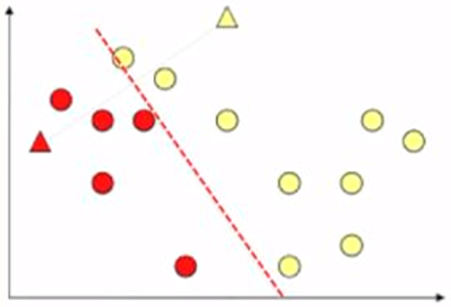
To run this K-means algorithm, first we randomly initialize two points (plotted as the red and yellow triangles in the figure below) as two cluster centroids.
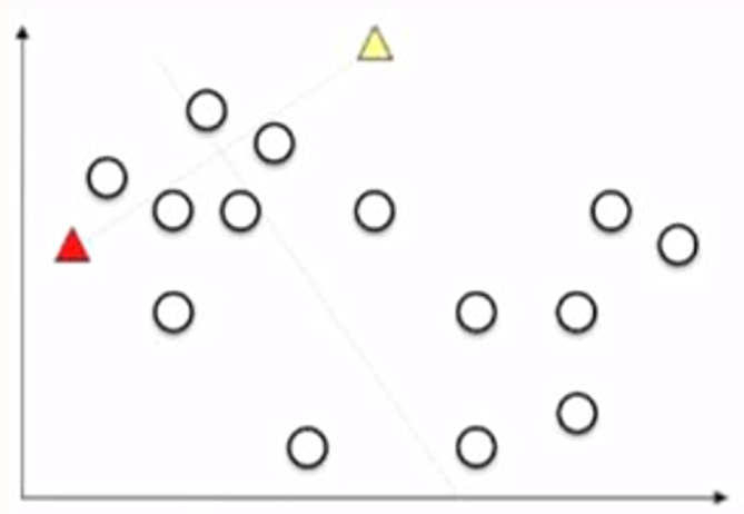
Next, we assign each point into the cluster closer to it. As illustrated below, we use different colours to present different clusters. And we call them the red cluster and the yellow cluster.
Now we calculate the average of the points in each cluster (i.e., the white triangle in the figure below).
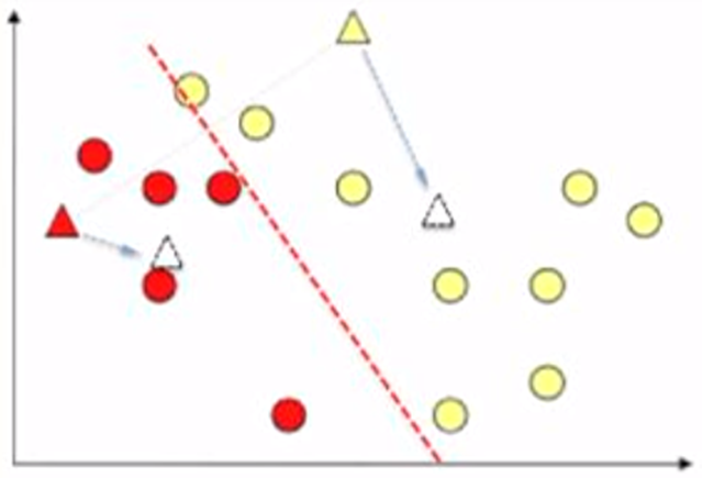
And update the cluster centroids to the average locations.
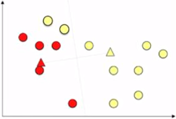
Then, use the updated centroid positions, assign the data points to either red or yellow cluster, depending on which cluster centroid the point closer to. As shown below, two points changed their colour, i.e., cluster.

Again, we update the centroid location to the average position of the points in each cluster.
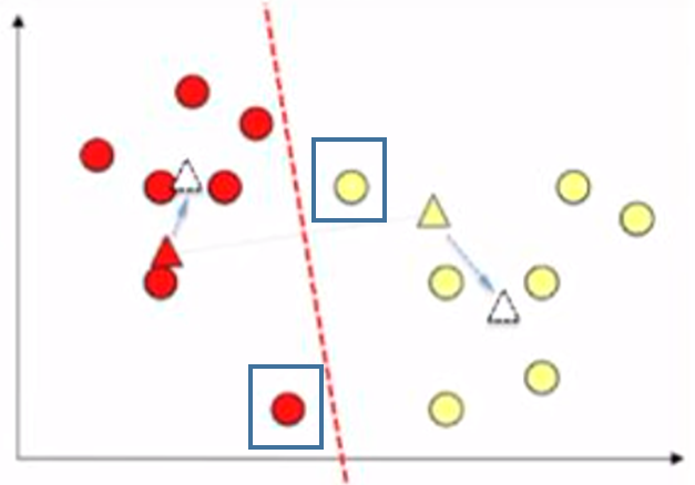
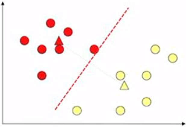
And re-assign the cluster to each point, two points changed their cluster in this iteration. Again we calculate the average position of the points in each cluster.
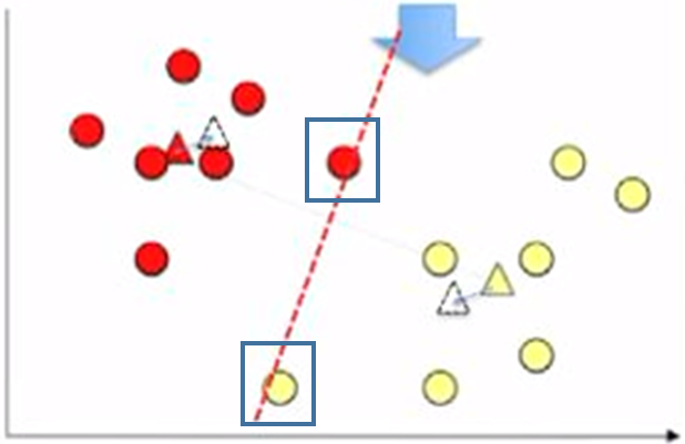
And move the centroids to the average position. Using the updated centroid location assign the cluster to the points, there is no change in the clusters: it is converged. And we have the 2 clusters.
-
Further reading
Machine Learning on 🔗 www.coursera.org by Andrew Ng
Han Jiawei, Kamber M., Pei J., Data Mining: Concepts and Techniques, Elsevier Inc., 2012