-
1. Introduction
This unit introduces indices, also known as powers or exponents. Indices provide a shorthand method for representing the repeated multiplication of an expression by itself. A good understanding of indices, and the associated laws of indices, is essential when it comes to applying algebraic manipulation to simplify and solve mathematical expressions and equations.
The laws of indices are introduced for integer and fractional exponents before applying these laws to simplify expressions and solve equations involving exponents. Graphs of exponential functions are presented to highlight the concepts of exponential growth and decay. The section closes with a brief look at basic mathematical models of growth and decay in real-world applications.
Links to further resources at the Mathcentre and Khan Academy websites are located at appropriate locations throughout this unit.
-
2. What are indices?
If required further resources on this topic can be found at:
🔗 http://www.mathcentre.ac.uk/topics/algebra/powers/
and
When a number is multiplied by itself several times we can represent the expression by introducing superscript notation where the number of times the multiplication is carried out appears as the superscript. The superscript is called the index.
Example 1
(i) $ 6 \times 6 = 6^2$ here $2$ is the index (power) and we read as “six raised to the power two”, or “six squared”
(ii) $ 6 \times 6 \times 6 = 6^3 $ here $3$ is the index (power) and we read as “six raised to the power three”, or “six cubed”
Note: We call the expression that we are raising to the power the base. Here the base is $6$.
End of Example 1Example 2
Indices appear in formulae for calculating physical quantities such as area and volume.
(i). the area of a square of side length $x$ metres is, $x × x = x^2$ (square metres).
(ii). the area of a circle of radius $r$ centimetres is, $ \pi \; r^2 $ (square centimetres).
(iii). the volume of a cube of side length $y$ metres is, $y × y × y = y^3$ (cubic metres).
(iii). the volume of a sphere of radius $r$ centimetres is, $ {\Large\frac{4}{3}} \; \pi \; r^3$ (cubic centimetres).
End of Example 2Example 3
Scientific notation provides us with an easy way for writing very large, or very small, numbers. In scientific notation we have:
(i). $ 3600000 = 3.6 \times 10^6 $
(ii). $ 0.0051 = 5.1 \times 10^{-3}$
(iii). $ 0.000078 = 7.8 \times 10^{-5}$
End of Example 3Example 4
A computer algorithm that loops as follows:
for $i = 1$ to $n$
for $j = 1$ to $n$
<perform action>
next $j$
next $i$
goes around the loop $n \times n$ times = $n^2$ times.
Indices therefore feature in a wide range of day-to-day calculations and there are associated rules that apply when performing calculations involving indices.
End of Example 4 -
3. The Laws of Indices
Law 1: If expressions with the same base are multiplied, the indices are added.
Example 5
(i). $ a^3 \times a^2 = a^{3+2} = a^5$
(ii). $ 4^9 \times 4^6 = 4^{9+6} = 4^{15} $
(iii). $ 2^6 \times 2^{11} = 2^{6+11} = 2^{17} $
in general $ \class{outbox}{a^m \times a^n = a^{m+n}} $
End of Example 5Law 2: If expressions with the same base are divided, the index of the denominator is subtracted from the index of the numerator.
Example 6
(i). $ {\Large\frac{a^6}{a^4}} = a^{6-4} = a^2 $
(ii). $ {\Large\frac{5^{16}}{5^7}} = 5^{16-7} = 5^9 $
(iii). $ {\Large\frac{7^9}{7^3}} = 7^{9-3} = 7^6 $
in general, $ \class{outbox}{{\Large\frac{a^m}{a^n}} = a^{m-n}}$
End of Example 6Law 3: If an expression involving a power is raised to a further power, the indices are multiplied together:
Example 7
(i). $ (a^3)^2 = a^{3 \times 2} = a^6 $
(ii). $ (3^8)^7 = 3^{8 \times 7} = 3^{56} $
(iii). $ (4^5)^6 = 4^{5 \times 6} = 4^{30} $
$ \class{outbox}{(a^m)^n = a^{m \times n} = a^{mn}}$
This law can actually be derived from Law1. For example from (i) above,
$$ (a^3)^2 = a^3 \times a^3 = a^{3+3} = a^6. $$
Hence, we are able to simplify expressions like the square of a cube.
End of Example 7Law 4: Zero index. Any number to the power $0$, except $0$, equals $1$.
Example 8
$ {\Large\frac{a^2}{a^2}} = a^{2-2} = a^0$ by law 2. $ (a \neq 0) $
However, $ {\Large\frac{a^2}{a^2}} = 1 $ as any number (except $0$) divided by itself equals $1$.
Hence, we must have that
$ \class{outbox}{a^0 = 1, \; a \neq 0 }$
End of Example 8Law 5: The product of two different expressions raised to a power.
Example 9
$ (2 \times 4)^3 = (2 \times 4) \times (2 \times 4) \times (2 \times 4) $
$ = (2 \times 2 \times 2) \times (4 \times 4 \times 4) $
$ =\;$$2^3\times4^3$
in general $ \class{outbox}{(ab)^n = a^nb^n }$
End of Example 9Law 6: The quotient of two different expressions raised to a power.
Example 10
$$ \Big(\frac{2}{3}\Big)^4 = \frac{2 \times 2 \times 2 \times 2}{3 \times 3 \times 3 \times 3} = \frac{2^4}{3^4} $$
In general
$$ \class{outbox}{\Big(\frac{a}{b}\Big)^n = \frac{a^n}{b^n}} $$
Hence, we apply the power to both expressions.
End of Example 10Example 11
Use the laws of indices to simplify each of the following:
(i). $ 2^2 \times 2^5 = 2^{2+5} = 2^7 = 128 $
(ii). $ {\Large\frac{2^4}{2^3}} \times 2^{4-3} = 2^1 = 2$
(iii). $ (4^2)^2 = 4^{2 \times 2} = 4^4 = 256$
(iv). $ \Big({\Large\frac{2}{3}}\Big)^3 = {\Large\frac{2^3}{3^3}} = {\Large\frac{8}{27}}$
(v). $ (4 \times 5)^3 = 4^3 \times 5^3 = 64 \times 125 = 8000 $
(vi). $ {\Large\frac{6^3 \times 6^4}{6^7}} = {\Large\frac{6^{3+4}}{6^7}} = {\Large\frac{6^7}{6^7}} = 6^{7-7} = 6^0 = 1 $
(vii). $ (2x)^3 = 2^3x^3 $
(viii). $ \Big({\Large\frac{3x}{4y}}\Big)^2 = {\Large\frac{3^2x^2}{4^2y^2}} = {\Large\frac{9x^2}{16y^2}} $
(ix). $ (3x^3y^4)(4x^2y^5) = 3x^3y^44x^2y^5 $
$ = 12x^{3+2}y^{4+5} $
$= 12x^5y^9$(x). $ (2a^2b^3c)^4 \;\; = (2)^4(a^2)^4(b^3)^4(c^1)^4 $
$ =2^4a^{2 \times 4}b^{3 \times 4}c^4 $
$ = 16a^8b^{12}c^4$(xi). $ {\Large\frac{((2x)^2)^3(2)}{2^7x^6}} = {\Large\frac{(2^2x^2)^3(2)}{2^7x^6}} $
$ = {\Large\frac{(2^6x^6)(2)}{2^7x^6}} $
$ = {\Large\frac{2^7x^6}{2^7x^6}} $
$ = $$\class{double}{1} $We now turn our attention to look at cases where the exponents are negative and/or fractional.
End of Example 11Law 7: Negative indices.
To avoid division by zero we must restrict the base number to take only non-zero real values.
Example 12
$$ \frac{a^2}{a^5} = \frac{a \times a}{a \times a \times a \times a \times a} = \frac{1}{a \times a \times a} = \frac{1}{a^3} \;\;\; (a \neq 0) $$
However, from Law 2 we have that $ {\Large\frac{a^2}{a^5}} = a^{2-5} = a^{-3} $
Hence, we must have that $ {\Large\frac{1}{a^3}} = a^{-3}$
in general $ \class{outbox}{{\Large\frac{1}{a^n}} = a^{-n} (a \neq 0).} $
or equivalently $ \class{outbox}{{\Large\frac{1}{a^{-n}}} = a^n (a \neq 0).} $
This law enables us to move expressions from the denominator to the numerator.
End of Example 12Law 8: Fractional indices.
Example 13
(i). From Law 1 we can write $ a^{1/2} \times a^{1/2} = a^1.$
We know that $ \sqrt{a} \times \sqrt{a} = a^1$
Hence, we conclude that $ a^{1/2} = \sqrt{a} $
The symbol $\sqrt{a} $ represents the square root of $a$, i.e. the number that when multiplied by itself returns the original number, $a$.
Note however that every number has a positive and a negative square root. For example,
$ \sqrt{4} \times \sqrt{4} = 2 \times 2 = 4 $ and $ \sqrt{4} \times \sqrt{4} = (-2) \times (-2) = 4$.
In our work, unless otherwise stated, we will work with the positive square root.
(ii). From Law 1 we can write $ a^{1/3} \times a^{1/3} \times a^{1/3} = a^1 $.
We know that $ \sqrt[3]{a} \times \sqrt[3]{a} \times \sqrt[3]{a} = a^1 $.
Hence, we conclude that $ a^{1/3} = \sqrt[3]{a} $, i.e. the cube root of $a$.
In general, $ \class{outbox}{a^{1/n} = \sqrt[n]{a}}$
The number in the denominator of the index specifies the root we are calculating.
End of Example 13Example 14
(i). Now consider $ a^{1/3} \times a^{1/3} = (a^{1/3})^2 = a^{2/3}$.
Also, $ \sqrt[3]{a} \times \sqrt[3]{a} = (\sqrt[3]{a})^2$.
Hence, we conslude that $ a^{2/3} = (\sqrt[3]{a})^2 $
The expression, $a^{2/3}$ means the square of the cube root of $a$.
Note that in the exponent the number in the denominator (3) is the root and the number in the numerator (2) is the power.
in general $ \class{outbox}{a^{m/n} = (a^{1/n})^m = (\sqrt[n]{a})^m }$ or $ \class{outbox}{ a^{m/n} = (a^m)^{1/n} = \sqrt[n]{a^m}}$.
End of Example 14Summarising the laws we have:
1. $ a^ma^n = a^{m+n} $
2. $ {\Large\frac{a^m}{a^n}} = a^{m-n}$
3. $ (a^m)^n = a^{mn} $
4. $ a^0 = 1$
5. $ (ab)^n = a^nb^n $
6. $\Big( {\Large\frac{a}{b}}\Big)^n = {\Large\frac{a^n}{b^n}} $
7. $ a^{-n} = {\Large\frac{1}{a^n}}\; \text{and}\; {\Large\frac{1}{a^{-n}}} = a^n $
8. $ a^{1/2} = \sqrt{a} \; \text{and} \; a^{1/n} = \sqrt[n]{a} $
$ a^{m/n} = (\sqrt[n]{a})^m \; \text{and}\; a^{m/n} = \sqrt[n]{a^m}$
These results will be needed in both the expansion and simplification of algebraic expressions as illustrated in the following examples.
Example 15
(i). $ {\Large\frac{4x^2y^{-6}}{3x^{-5}y^6}} = {\Large\frac{4}{3}}(x^2y^{-6})(x^5y^{-6}) $
$ ={\Large\frac{4}{3}} x^{2+5}y^{-6-6} $
$ ={\Large\frac{4}{3}}x^7y^{-12} $
$ ={\Large\frac{4x^7}{3y^{12}}}$(ii). $ {\Large\frac{2p^4q^{-3}}{7p^{-2}q^{-6}}} = {\Large\frac{2}{7}}(p^4q^{-3})(p^2q^6) $
$ = {\Large\frac{2}{7}}p^{4+2}q^{-3+6} $
$ = {\Large\frac{2}{7}}p^6q^3$(iii). $ \Big({\Large\frac{5x^6y^2}{x^2y^{-5}}} \Big)^4 = {\Large\frac{5^4x^{6 \times 4}}y^{2 \times 4}}{x^{2 \times 4}y^{-5 \times 4}} $
$ = {\Large\frac{5^4x^{24}y^8}{x^8y^{-20}}} $
$ = 5^4x^{24}y^8x^{-8}y^{20} $
$ = 625x^{24-8}y^{8+20} $
$ = 625x^{16}y^{28}$(iv). $ r^4s^{-7}(6r^2s)^{-3} = r^4s^{-7}6^{-3}r^{-6}s^{-3} $
$ = r^{4-6}s^{-7-3}6^{-3} $
$ = r^{-2}s^{-10}6^{-3} $
$ = {\Large\frac{1}{r^2s^{10}6^{3}}} $
$ = {\Large\frac{1}{216r^2s^{10}}} $(v). $ {\Large\frac{p^{1/4}q^{4/3}r^2}{p^{3/4}q^{1/3}r^{1/2}}} = p^{1/4}p^{-3/4}q^{4/3}q^{-1/3}r^2r^{-1/2} $
$ = p^{-1/2}q^1r^{3/2} $
$= {\Large\frac{qr^{3/2}}{p^{1/2}}}$End of Example 15Example 16
Evaluate each of the following expressing your answer as an exact numerical value.
(i). $ 8^{2/3} = (8^2)^{1/3} = \sqrt[3]{8^2} = \sqrt[3]{64} = \class{double}{4} $
(ii). $ 16^{-1/4} = {\Large\frac{1}{16^{1/4}}} = {\Large\frac{1}{\sqrt[4]{16}}} = $$1$$\;{\Large\frac{1}{2}}$(iii). $ 27^{2/3} = (3^3)^{2/3} = 3^{3 \times 2/3} = 3^2 = \class{double}{9} $
Examples (i) - (iii) produced exact solutions in the form of whole numbers or fractions. However, a number such as $ \sqrt{7} = 7^{1/2} $ does not produce an exact solution and evaluates to give an infinite decimal which to four decimal places is $2.6456$. We now take a brief look at numbers of this form.
End of Example 16 -
4. Surds
A number that can be expressed as a ratio, $ {\Large\frac{m}{n}} $, of two integers $m$ and $n$, with $n \neq 0$, is called a rational number. Any number whose root cannot be expressed as a rational number is called a surd. For example, $ \sqrt{2} $ and $ \sqrt[3]{5} $ are both surds as when evaluated they produce infinite decimals, i.e. they cannot be expressed as the ratio of two integers.
On the other hand, $ \sqrt{4} = 2 = {\Large\frac{2}{1}}\; \text{and}\; \sqrt[4]{{\Large\frac{16}{81}}} = \Big({\Large\frac{16}{81}}\Big)^{1/4} = {\Large\frac{16^{1/4}}{81^{1/4}}} = {\Large\frac{2}{3}} $ are not surds.
Closely related to the Laws of Indices are the Laws of Surds and the four main laws are listed below.
1. $ \sqrt{a} \times \sqrt{b} = a^{1/2} \times b^{1/2} = (ab)^{1/2} = \sqrt{ab} $ (Multiplication of surds)
2. $ {\Large\frac{\sqrt{a}}{\sqrt{b}}} = {\Large\frac{a^{1/2}}{b^{1/2}}} = \Big({\Large\frac{a}{b}}\Big)^{1/2} = \sqrt{{\Large\frac{a}{b}}} $ (Division of surds)
3. $ m\sqrt{a} + n\sqrt{a} = (m + n)\sqrt{a} $ (Addition of surds)
4. $ m\sqrt{a} - n\sqrt{a} = (m - n)\sqrt{a} $ (Subtraction of surds)
Example 17
Simplify the following:
(i). $\sqrt{50} = \sqrt{25 \times 2} = \sqrt{25}\sqrt{2} =\; $$5\sqrt{2}$
(ii). $ \sqrt[3]{{\Large\frac{216}{125}}} = {\Large\frac{\sqrt[3]{216}}{\sqrt[3]{125}}} = $$1$$\; {\Large\frac{6}{5}} $
(iii). $ 3\sqrt{7} + 4\sqrt{7} - 2\sqrt{7} = ( 3 + 4 - 2)\sqrt{7} = \;$$ 5\sqrt{7}$
(iv). $ \sqrt{12u^6} = \sqrt{12}\sqrt{u^6} = \sqrt{4 \times 3}\; u^3 = \sqrt{4}\sqrt{2}\; u^3 =\; $$ 2\sqrt{3}\; u^3$
(v). $ \sqrt{\sqrt{4x^4}x^6y^8} = [(4x^4)^{1/2}x^6y^8]^{1/2} $
$ = (4x^4)^{1/4}x^3y^4 $
$ = 4^{1/4}x^1x^3y^4 $
$ = $$ \sqrt{2}\; x^4y^4$End of Example 17 -
5. Solving exponential equations using the laws of indices
If required further resources on this topic can be found at
📹 Solving exponential equations using exponent properties
The next block will describe how to solve exponential equations using logarithms but for now we look at solving specific types of these equations using the laws of indices.
Example 18
Solve the following equations for $x$.
(i). $ 9^{x-1} = 3^{3x+1}$
Both sides of the equation must be expressed in terms of the same base number.
Then compare the exponents and solve for $x$. We have
$9^{x-1} = 3^{3x+1} $
$(3^2)^{x-1} = 3^{3x+1} $ (base number on both sides must be 3)
$3^{2x-2} = 3^{3x+1}$ (both sides now have 3 as the base number)
$2x - 2 = 3x + 1$ (equate exponents)
$x = -3$ (solve the $x$)
(ii). $6^{2x-1} = 1 $
$ 6^{2x-1} = 6^0 $ (base number on both sides is now 6)
$ 2x - 1 = 0 $ (equate exponents)
$x = 1 ∕ 2$ (solve the $x$)
(iii). $ {\Large\frac{3^x}{81}} = 81 $
$ 3^x = 81^2 $
$ 3^x = (3^4)^2$
$ 3^x = 3^8 $
$x = 8$
(iv). $2^{x^2-7} = 4^{x + 4} $
$2^{x^2-7} = (2^2)^{x+4} $
$2^{x^2-7} = 2^{2x+8} $
$ x^2 - 7 = 2x + 8 $
$ x^2 - 2x - 15 = 0 $
$ (x - 5)(x + 3) = 0 $
$x = 5$ or $x = -3$
(v). $ \Big({\large\frac{1}{3}}\Big)^{2x+7} = 243 $
$ (3^{-1})^{2x+7} = 3^5 $
$ 3^{-2x-7} = 3^5$
$ -2x - 7 = 5 $
$x = - 6$
(vi). $ \Big(\frac{1}{16}\Big)^{x-3} - 23 = 1001 $
$ \Big({\Large\frac{1}{4^2}}\Big)^{x-3} = 1024$
$(4^{-2})^{x-3} = 4^5$
$4^{-2x+6} = 4^5$
$-2x + 6 = 5$
$-2x = -1$
$x = 1 ∕2$
End of Example 18 -
6. Modelling Examples
There are many modelling situations requiring the development of indicial equations. Many of these are solved using logarithms, which are covered in the next unit. Here we confine ourselves to examples that do not require logarithms in their solution.
Example 19 (Compound Interest)
The money in an account grows by 4% per annum. Assume the account starts with £2000.
(i). Derive a general expression for the amount in the account in $n$ years.
(ii). How much will be in the account in 10 years?
Solution
(i). We can derive an expression for the amount in the account after a given number of years by generalising from a few cases.
Let $x_n$ be the amount in the account at the beginning of year $n$.
Choose the initial year to be year $0$ so that $x_0 = 2000$.
The amount in the account at the beginning of year 1 is,
$x_1 = 2000 + 0.04 \times 2000 = (1 + 0.04) \times 2000 = 2000(1.04)$.
This is the initial amount in the account plus the accrued interest.
Now consider the amount at the beginning of year 2.
$x_2 = x_1 + 0.04x_1 = 1.04x_1$
We already have an expression for $x_1$, and so
$x_2 = (1.04)(1.04)2000 = 2000(1.04)^2$
This generalises to $x_n = 2000(1.04)^n$.
We have derived an indicial formula for the amount in the account at the start of year $n$:
$x_n = 2000(1.04)^n$.
(ii). To find the amount in the account after 10 years we set $n = 10$ in the formula derived in part (i), i.e.
$x_{10} = 2000(1.04)^{10} = $$\class{double}{£}$$\class{double}{2}$$\class{double}{9}$$\class{double}{6}$$\class{double}{0}$$\class{double}{.}$$\class{double}{4}$$\class{double}{9}$.
The above type of development is common in indicial modelling – you should make sure that you are comfortable with it.
End of Example 19Example 20 (Oil Extraction)
A newly discovered oilfield is believed to contain 10 billion barrels of crude oil. It will have oil removed from it at the rate of 9% per annum. Derive an expression for the amount of oil remaining in the field after $n$ years and use it to calculate how much will be in the field after 8 years. How much oil will be removed in the ninth year?
Solution
Denote the amount of oil (barrels) in the field at the end of year $n$ by $A_n$. For convenience we work in units of billions.
$A_0 = 10 $
$A_1 = (0.91)10$ (we have used $A_1 = A_0 - 0.09A_0 = (0.91)A_0$)
$A_2 = (0.91)^210$ (we have used $A_2 = A_1 - 0.09A_1 = 0.91A_1$
$= (0.91)(0.91)A_0 = (0.91)^2A_0)$In general we obtain an expression for the amount of oil remaining in the field after $n$ years as,
$A_n = (0.91)^nA_0$.
After 8 years the quantity $A_8 = (0.91)^8(10) = 4.70$ billion barrels. This is the amount of oil remaining in the field after 8 years.
After 9 years, $A_9 = (0.91)^9(10) = 4.28$ billion barrels remain in the field.
Hence, the quantity extracted during year 9 is the difference between these two values, i.e. $4.70 - 4.28 = 0.42$ billion barrels. (An alternative for this problem would be to take 9% of $A_8$).
End of Example 20 -
7. Exponential Functions
An exponential function is one that contains a variable exponent and is of the form
$y=a^x$$(a > 0, a \neq 1)$
The number $a$ is called the base and the number $x$ is the exponent.
Often an exponential function will be multiplied by a scaling constant, $k$ say, and the exponential function takes the form
$y=ka^x$$(a > 0, a \neq 1)$
7.1. Graphs of exponential functions
Note here that exponential functions grow far too fast to include a wide range for $x$ in the plots.
Example 21
Plot the functions, $ y = 2^x $ and $ y = 2^{-x} = {\Large\frac{1}{2^x}} $ on the same graph.
Solution
Using a calculator for selected $x$ values we create the table
$x$ $-4$ $-3$ $-2$ $-1$ $0$ $1$ $2$ $3$ $4$ $y=2^x$ $0.0625$ $0.125$ $0.25$ $0.5$ $1$ $2$ $4$ $8$ $16$ $y = 1/2^x$ $16$ $8$ $4$ $2$ $1$ $0.5$ $0.25$ $0.125$ $0.0625$ Now plot the graphs but restrict the $x$-interval to between $– 2$ and $2$ for clarity.
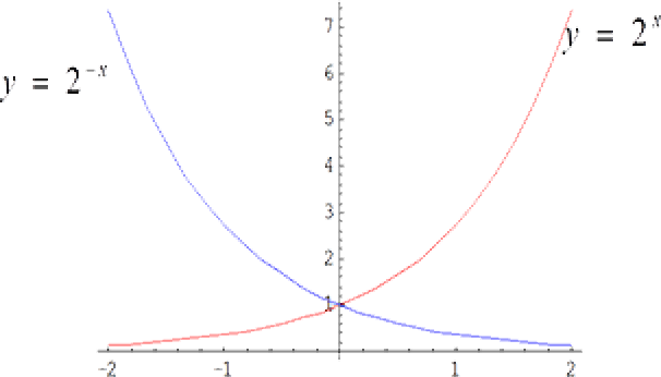
- Note the following:
- Both functions are positive for all values of $x$.
- Both graphs pass through the point $(0, 1)$.
- The graphs are mirror images of each other in the $y$-axis.
- The graph of $y = 2^x$ increases without bound with increasing $x$, i.e. it exhibits exponential growth.
- The graph of $y = 2^{-x}$ decreases rapidly with increasing $x$, i.e. it shows exponential decay. Note that the graph never reaches the $x$-axis.
End of Example 21Example 22
(i). The figure below shows the graphs of several exponential functions, $y = a^x, \; (a > 1)$.
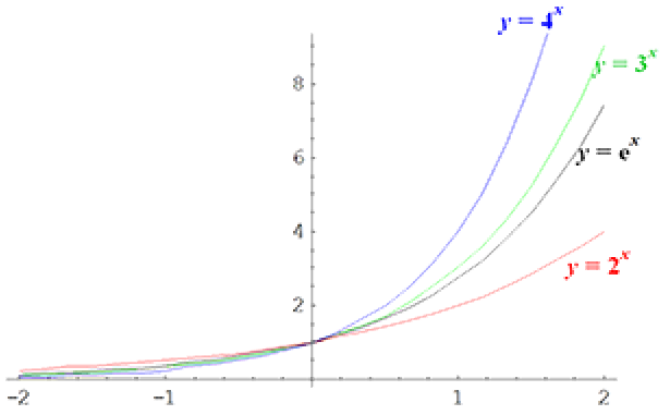
- Properties to note from the graph are:
- As $a > 1$ the functions all display exponential growth.
- The functions are positive for all values of $x$.
- In all cases as $x$ increases, $y$ grows very fast and keeps on growing.
- All graphs pass through the point $(0, 1)$.
One exponential function that occurs frequently when modelling real world phenomena uses the constant $e = 2.7182818...$ as its base. It occurs so often that it is often referred to as THE exponential function. The graph of $y = e^x$ is shown, as expected, sandwiched between the graphs of $y = 2^x$ and $y = 3^x$ as $2 < e < 3$.
(ii). The figure below shows the graphs of several exponential functions, $y = a^{-x}, (a > 1)$.
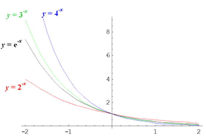
- Properties to note from the graph are:
- As $a > 1$ the functions all display exponential decay.
- In all cases as $x$ increases, $y$ decreases rapidly, and keeps on decreasing, but never actually reaches $y = 0$, i.e. the $x$-axis.
- The functions are positive for all values of $x$.
- All graphs pass through the point $(0, 1)$.
End of Example 22 -
8. Applications of exponential growth and decay
Here we present, through worked examples, mathematical models of exponential growth and decay occurring in real-world applications.
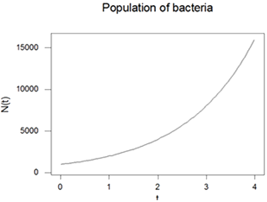
Example 23 (Population Growth)
Suppose that the number of bacteria in a certain culture doubles every hour. Assuming that the culture has 1000 bacteria to start with:
(i). determine a formula that gives the number of bacteria, $N(t)$, in the culture after $t$ hours.
(ii). determine the number of bacteria in the culture after 4 hours.
Solution
Here we assume that the bacteria have enough space and a food source to assist continued growth.
(i). Let $N(t)$ denote the number of bacteria in the culture after $t$ hours
After $t = 0\; \text{hours}: N(0) = 1000$
After $t = 1\; \text{hour}: N(1) = (1000)(2) = 2000$
After $t = 2\; \text{hours}: N(2) = [(1000)(2)](2) = (1000)(2^2) = 4000$
After $t = 3\; \text{hours}: N(3) = [(1000)(2)(2)](2) = (1000)(2^3) = 8000$
Examining the structure we have:
$N(0) = 1000 = (1000)(2^0)$
$N(1) = 2000 = (1000)(2^1)$
$N(2) = 4000 = 1000 (2^2)$
$N(3) = 8000 = 1000 (2^3)$
Hence, $N(t) = 1000(2^t)$ giving the general formula for the number of bacteria in the culture after $t$ hours.
(ii). After 4 hours the number of bacteria in the culture is: $N(4) = 1000(2^4) = 16000$.
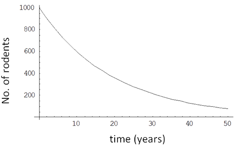
End of Example 23Example 24 (Population Decline)
On a particular island there are currently 1000 rodents. Various studies have shown that the size of this population has been decreasing at an average rate of 5% per annum for the past decade.
(i). determine a formula for $N(t)$, the number of rodents after $t$ years.
(ii). determine how many rodents will be on the island in 10 years time.
Solution
Here we assume that the rate of decline of 5% will continue.
(i). If 5% of the population is lost after one year then 95% of the population is left.
Let $N(t)$ denote the number of rodents on the island after $t$ years.
After $t = 0\; \text{years}: N(0) = 1000$
After $t = 1\; \text{year}: N(1) = (1000)(1 - 0.05)$
$= (1000)(0.95)$After $t = 2\; \text{years}: N(2) = N(1)(1 - 0.05)$
$= N(1)(0.95)$
$= (1000)(0.95)(0.95)$
$= (1000)(0.95)^2$After $t = 3\; \text{years}: N(3) = N(2)(1 - 0.05)$
$= N(2)(0.95)$
$= (1000)(0.95)^2(0.95)$
$= (1000)(0.95)^3$Continuing in this way the number of rodents in the population after $t$ years is given by
$N(t) = (1000)(0.95)^t$.
(ii). The number of rodents after 10 years is given by:
$N(10) = (1000)(0.95)^{10}$
$= 599$ to the nearest whole number.Assuming that the annual average decline remains at 5%, there will be 599 rodents on the island in 10 years.
 End of Example 24
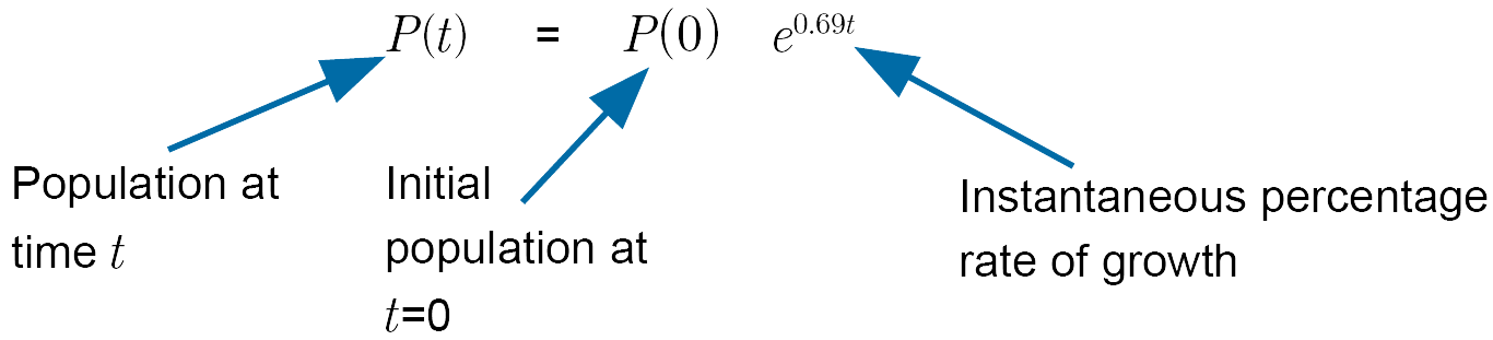
Average and Instantaneous Percentage Rates
In the last two examples we have used the average percentage rate of increase or decrease. This is not the same as the instantaneous percentage rate of increase or decrease.
An average percentage rate of change looks at the rate of change over an interval between two particular points in time. An instantaneous percentage rate of change looks at the rate of change at one particular point in time.
It is relatively straightforward to show for the example on population growth (Example 23) that the instantaneous percentage rate of growth of the bacteria population is approximately 69% per hour. (The necessary calculations however require knowledge of calculus which is beyond the scope of this course).
-
9. Exponential Functions with base $e$
The mathematical model from Example 23 for the average population percentage growth rate can we written as an instantaneous percentage growth rate model as
On the other hand if a population has some initial size, $P(0)$, and the population is declining exponentially at an instantaneous percentage rate of 5% per year as in Example 24, then the mathematical model is given by
$P(t) = P(0)e^{-0.05t}$
Note the negative sign in the exponential to account for the decline in the population.
Example 25
A bacterial culture follows a growth model given by
$P(t) = P(0)e^{0.2554t}$
where $P(0)$ is the initial population of 3000 and $P(t)$ is the size of the population at time $t$ hours.
(i). Determine the population size at time $t = 4$ hours.
(ii). If the culture medium can only support a population of 50000 determine the time, $T$ say, when the population reaches this value.
Solution
(i). Here $P(0) = 3000$ and $t = 4$ so the formula becomes
$P(4) = 3000e^{0.2554\times4}$
$= 8333$ bacteria to the nearest whole number.Hence, after 4 hours the population size has grown to approximately $8333$ bacteria.
(ii). Setting $t = T$ we require the value of $T$ for which $P(T) = 50000$.
Hence, $50000 = 3000e^{0.2554T}$ which simplifies to give
$e^{0.2554T} = {\Large\frac{50}{3}}$.Here we need knowledge of logarithms to solve for $T$ and this topic will be presented in the next unit.
End of Example 25 -
Summary
- This unit introduced indices and exponentials. You should now be able to:
- apply the laws of indices to simplify algebraic expressions
- apply the laws of indices to solve equations involving exponents
- sketch exponential functions
- derive and solve basic mathematical models of exponential growth and decay.
Now attempt the tutorial questions and the Maple exercises available on GCU Learn.
The next unit introduces the topic of logarithms.