-
Scalability
Scalability and its impact a fundamental issue in the cloud.
Several related lectures:-
1.Reliability and Scalability (this one)
2.Architecture and Scaling Techniques
3.Data Scalability
4.Consistency
Overview
- Reliability
- Faults, Failures and Availability
- The Bathtub Curve Model
- Scalability
- Vertical and Horizontal Scalability
- Measuring Scalability
- Ahmdal’s Law
- Universal Scalability Law
Reliability and Scalability
- In the cloud these are related.
- reliability is about avoiding failure in the presence of individual component faults
- scalability is about maintaining performance as demand grows
Both have to be addressed by architecting applications correctly.
Both mean some of the same techniques have to be used e.g. replication.
-
Reliability
The cloud is a large-scale distributed system made out of many commodity components – individual solution component faults (hardware and/or software) will be commonplace.
- AWS say:-
- “the reality is that most software systems will degrade over time. This is due in part to any or all of the following reasons:
- Software will leak memory and/or resources. This includes software that you have written, as well as software that you depend on (e.g., application frameworks, operating systems, and device drivers).
- File systems will fragment over time and impact performance.
- Hardware (particularly storage) devices will physically degrade over time.”
🔗 Building Fault-Tolerant Applications on AWS
Faults and Failures
AWS go on to say:-
“Disciplined software engineering can mitigate some of these problems, but ultimately even the most sophisticated software system is dependent on a number of components that are out of its control (e.g., operating system, firmware, and hardware). Eventually, some combination of hardware, system software, and your software will cause a failure and interrupt the availability of your application.”
So all the time we have a multitude of unavoidable faults happening and under these conditions we have to architect our cloud application to try to avoid failure.
- Fault tolerance is achieved by designing the system with a high degree of hardware redundancy.
- but the software has to be designed to use it
- basically replicated instances of services
Note that some outages may be caused by upgrades in progress rather than faults or by hardware or software overloading.
eBay:
“Design to fail”: implement automated fault detection and a degraded “limp mode”
- The system should be distributed into fault domains (or fault zones).
- a fault domain is a set of hardware components – computers, switches, and more – that share a single point of failure
- should separate service instances into separate fault domains thereby improving reliability
above diagram is really modelling fault occurrence i.e. independent faults of a particular hardware component type
note difference between blue and commonly (naively) assumed green lines
Measuring Reliability
- MTBF
- mean time between failures
- really meaning between component faults as defined previously...
- generally used to calculate the probability of failure for a single solution component
- average time interval, usually expressed in thousands or tens of thousands of hours that elapses before a component fails and requires service
- a basic measure of a system’s reliability and is usually represented as units of hours
- MTTR
- mean time to repair
- the average (expected) time taken to repair a failed component
- again usually represented as units of hours
- Availability
- a measure of the reliability of a service
- $\rho$ is the probability that the service is unavailable either through component failure or network partition
- calculated as a fraction of the time an individual service instance is unavailable i.e. dimensionless
$\rho = MTTR / (MTBF + MTTR)$ - availability of the service is defined as $1 - \rho$
- availability as a quantity is popularly given as the equivalent percentage of uptime i.e. 99.5% rather than 0.995
- Availability of replicated services
- the overall reliability of a system composed of set of replicated, identical and independent service instances in a parallel configuration
- availability of a system of $n$ replicated services is $1 - \rho ^n$
- where probability of all instances having failed at any instant is $\rho ^n$
- Availability of dependent services
- when two (or more) connected services are required to be available together in order for the system to be available
- i.e. if any of these services fail the system is considered to be unavailable
- aggregate availability of a system of connected dependent services is
$(1 - \rho^i) * (1 - \rho^j) * (1 - \rho^k) \dots$ - where $i$, $j$ and $k$ etc. are the replication factors of the separate sub-systems of services as above
Availability
- Availability is often quoted in “nines”.
- e.g. a solution with an availability level of "three 9s" is capable of supporting its intended function 99.9 percent of the time—equivalent to an annual downtime of 8.76 hours per year on a $24 \times 365$ basis.
- Gartner suggest:-
- high availability = 99.9% availability – “three 9s”
- normal commercial availability = 99 – 99.5% availability –87.6 – 43.8 hours/year downtime
“AWS will use commercially reasonable efforts to make Amazon EC2 and Amazon EBS each available with a Monthly Uptime Percentage of at least 99.95%”...
Should not underestimate the importance put on high application availability by modern business.
X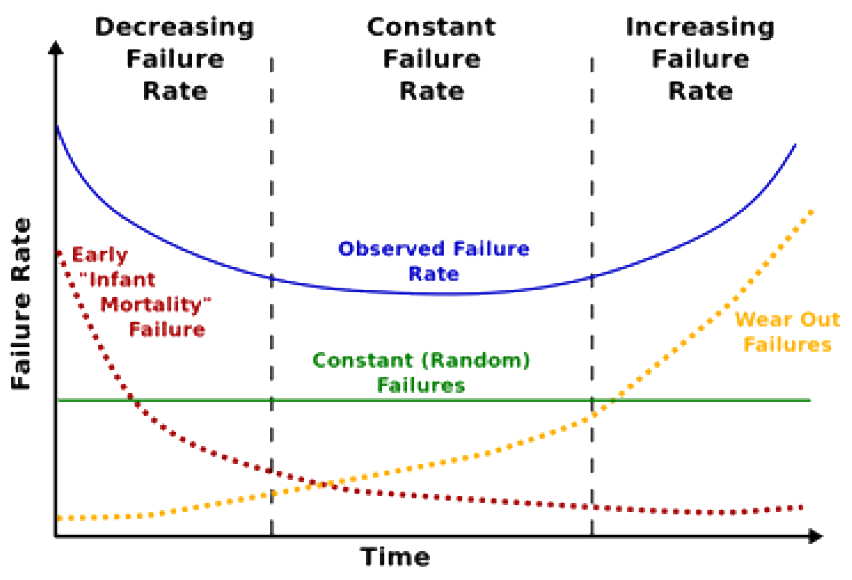
-
Scalability
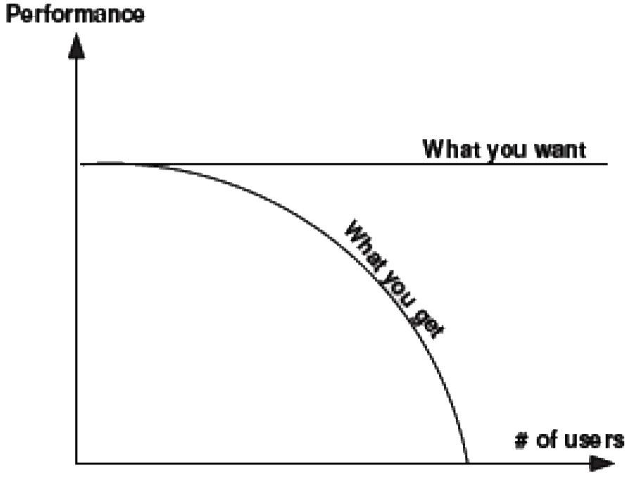
Definition: A system is said to be scalable if it can handle the addition of users and resources without suffering a noticeable loss of performance or increase in administrative complexity.
- Factors:
- number of users/objects/machines in the system (congestion, load, failure points and probability of failure, heterogeneity)
- distance between the parts of the system (hard to manage, latency)
- number of organisations that have administrative control over the system (heterogeneity, management issues)
Scalability Factor
Every component whether processors, servers, storage drives or load-balancers have some kind of management/operational overhead.
When attempting to increase the scale of a system by introducing new components or, increasing the capacity of existing ones, it is important to understand what percentage of the newly configured system is actually usable.
This measurement is called the scalability factor i.e. if only 95% of the expected total new processor power is available when adding a new CPU to the system, then the scalability factor is 0.95.
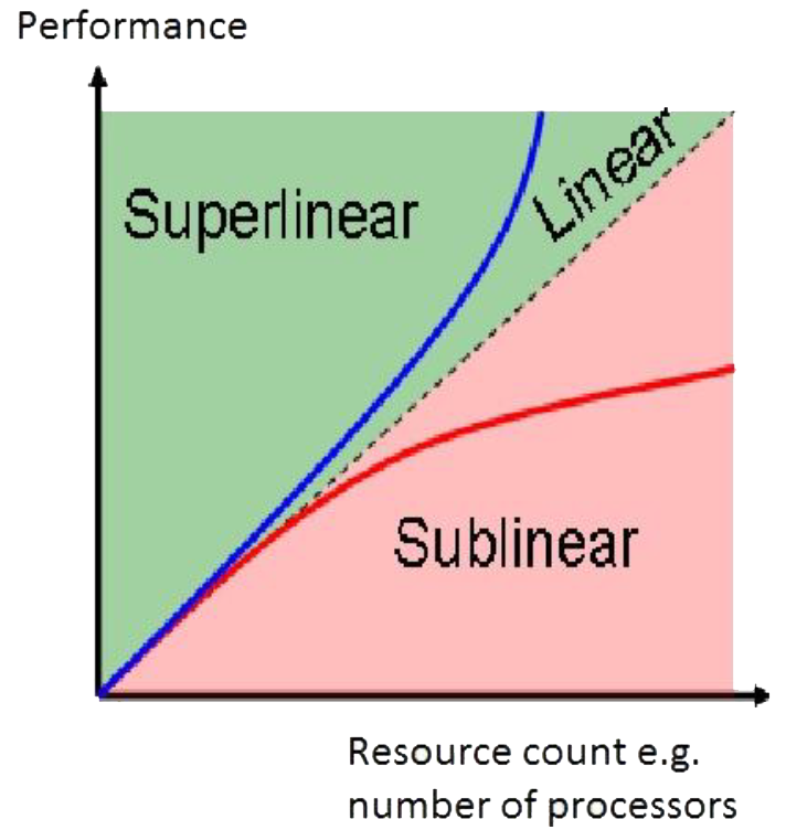
- We can further quantify scalability factor as:-
- linear scalability: the performance improvement remains proportional to the upgrade as far as you scale i.e. a scalability factor of 1.0.
- sublinear scalability: a scalability factor below 1.0. In reality some components will not scale as well as others. In fact the scalability factor may itself tail off as more resources are progressively added.
- sub-linear scalability likely to be the reality
- see section on Amdahl/USL at end
- superlinear scalability: although rare, it is possible to get better than expected ( > 1.0) performance increases e.g. some Hadoop cloud applications
- however Gunther has shown that this behaviour is exhibited at small scale only with a penalty as the systems gets larger
- negative scalability: if the application is not designed for scalability, it is possible that performance can actually get worse as it scales.
Scalability
There are two key primary ways of scaling architectures:-
Vertical Scalability: adding resource within the same logical unit to increase capacity. An example of this would be to add CPUs to an existing server, and more memory and/or expanding storage by adding hard drive on an existing RAID/SAN storage. Sometimes this is termed scaling up.
Horizontal Scalability: adding multiple logical units of resources and making them work as a single unit. Most clustering solutions, distributed file systems, load-balancers aid horizontal scalability. Usually this is achieved using less powerful machines than the single one used in vertical scalability above. Sometimes this is termed scaling out.
Cloud computing is a key example of horizontal scalability.
Vertical Scalability + and –
Often can be achieved without considering new architectural considerations and without changing application code +
Gets non-linearly more expensive as more resources added –
Better for building a solution for a future capped number of users
In reality the ability to scale vertically is limited.
Horizontal Scalability + and –
- Software has to be designed to be split horizontally –
- this can be hard!
- what this lecture’s really about...
Replica consistency a big issue –
More points of failure (hardware/network) –
Hardware cheaper (not necessarily cheap though) +
a driving factor
Better for building a solution to cater for many future concurrent users simultaneously.
A multi-tier/layer system may in fact lend itself to being split horizontally.
eBay:
“If you can’t split it, you can’t scale it”: eBay realised early on that anything which cannot be split into smaller components can’t be scaled!
-
Quantifying Scalability
Will look at how to measure the effectiveness of scaling i.e. to determine a cost/benefit analysis of adding hardware:-
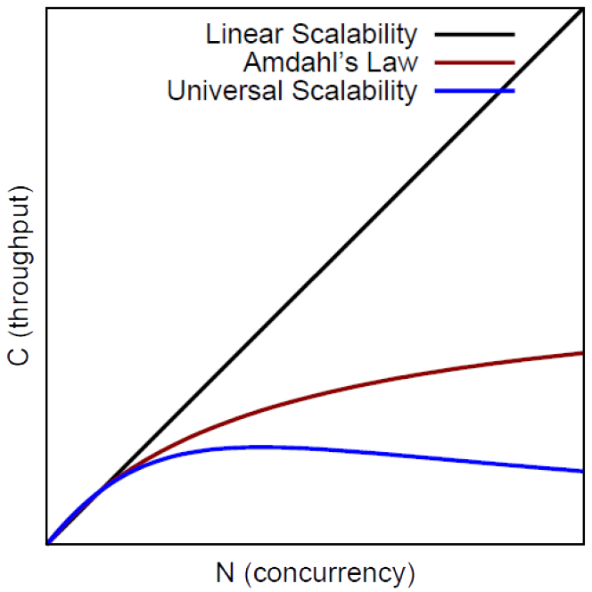
Amdahl’s Law: really a better measure for supercomputers and clusters involved in HPC (high-performance computing).
however an interesting insight into the limits of scalability
Universal Scalability Law: a more realistic measure of scalability in distributed systems taking into account overheads of communication and synchronisation.
Scaling by Adding More Cores
The clock speeds of microprocessors are not going to improve much in the foreseeable future.
The number of transistors in a microprocessor is still growing at a high rate.
one of the main uses of transistors has been to increase the number of computing cores the processor has
- However as cores are added the performance of the system does not scale linearly.
- governed by Amdahl’s Law and by the Universal Scalability Law
- a good example of sub-linear scalability
Here, for simplicity, think of 1 core VMs - so the unit of increasing parallel computation is a VM instance.
but this argument can be adapted/extended to multi-core processors or multi-processor VMs etc.
Quantifying Scalability
Speed-up $S$ measures the effectiveness of parallelization:
$$ S = \frac{T(1)}{T(N)}$$
$T(1)$: execution time of serial computation.
$T(N)$: execution time of $N$ parallel cores.
and of course $T(N) < T(1)$ so hence the arrangement of numerator and denominator
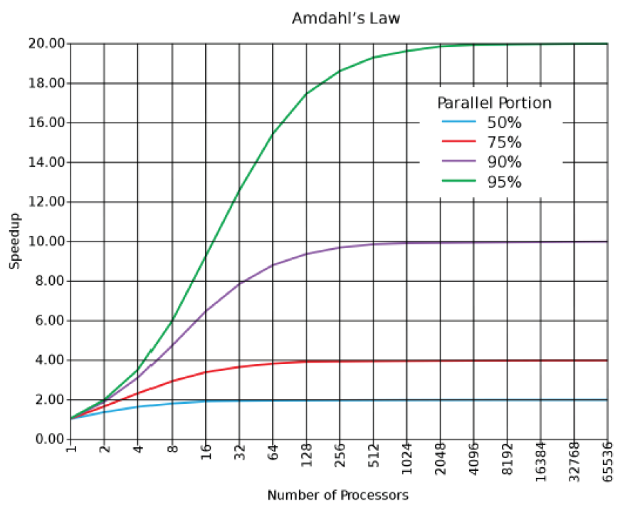
Amdahl's Law
(1). order to keep the ever increasing number of cores busy, the applications must be extremely parallel to exploit the benefits of increasing transistor counts.
(2). quantify this Amdahl's law states that for a given application contention $\sigma$ i.e. the proportion of the code that cannot be parallelised (remains serial), then the maximum speedup that can be achieved by using N cores is:-
$$ S = \frac{N}{1 + \sigma(N-1)} $$
- consequently $(1 - \sigma)$ is the proportion of a program that can be made parallel (i.e. benefit from parallelisation)
- notice the contention limits $S$ and what happens for large value $N$
Amdahl's Law - Cloud Context
- Andahl's law is an interesting basis for measuring scalability
- but it is ultimately "a law of diminishing returns"
- it was originally defined for use with large standalone computers solving hard mathematical problems
- By itself it is only applicable to certain workloads in the cloud as it does not model other factors such as network latency between nodes or synchronisation factors.
- e.g. good for embarrassingly parallelised applications
- little effort to distribute into many parallel tasks in separate VMs
- no (or little) dependency or communication between parallel task VMs
Universal Scalability Law (USL)
Gunther (2007/2015)
(1). A more realistic extension of Amdahl’s Law for general cloud applications.
(2). A new factor is included in equation:-
- coherence $(κ)$: the cost of consistency e.g. the time it takes to synchronise data in different nodes in a system or to introducing locking i.e. the penalty incurred to make resources consistent
In practice coefficient values for contention and coherence are determined experimentally from controlled experiments and then used to determine how well the system will scale with more hardware added.
- allows determination of optimal optimisation and system bottlenecks
$$ \frac{N}{1 + \sigma(N + 1) + kN(N-1)}$$
Better describes real systems as the performance degrades beyond an optimal point
If $κ = 0$ then USL reduces to Amdahl’s Law
If $\sigma = 0$ and $κ = 0$ then USL and Amdahl’s Law reduce to model linear scalability