-
10. Trees
In Section 3.5 we introduced a specialised graph called a tree. A tree is a connected graph with no cycles and occurs commonly as a data structure in computer science, playing a significant role in computer networks.
An important application when working with trees is the ability to search them for data they may hold. In this section we describe two algorithms for searching trees: depth first search (DFS) and breadth first search (BFS). These two algorithms have simple variations for searching digraphs and graphs but these are not followed up here.
10.1 Definition
A tree is a simple connected graph without cycles, i.e. an acyclic graph. We require that a tree is simple, meaning that it has no parallel (multiple) edges or loops.
For a “small” graph it is relatively easy to identify if it is a tree from its pictorial representation.
Example 29
The following are both trees:

A tree has at least two vertices of degree $1$. Vertices of degree $1$ are called leaves.
When working with trees, vertices are often called nodes.
End of Example 29Example 30
The following are not trees. The example on the left includes a cycle, $\{ \text{Bob}, \text{Liz}, \text{Jill}, \text{John}, \text{Bob} \}$, while the one on the right fails because it has parallel edges; it also fails because it contains a loop.
 End of Example 30
10.2 Rooted Trees
We now identify a particular class of tree known as a rooted tree. These trees have a special vertex called the root. Many algorithms on trees start at the root.
The existence of the root in a tree gives an implied direction to the edges of the tree, i.e. moving away from the root, from the upper level to the lower level. The structure of the rooted tree is highlighted in pictures by placing the root at the top and having the vertices hanging.
Example 31
Consider the following tree with root $C$:
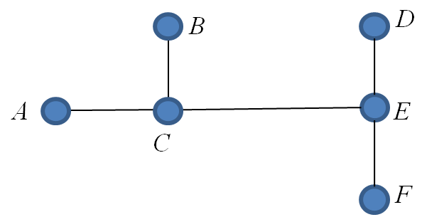
Using the vertex $C$ as a root we identify a direction on each edge changing it into an arc:
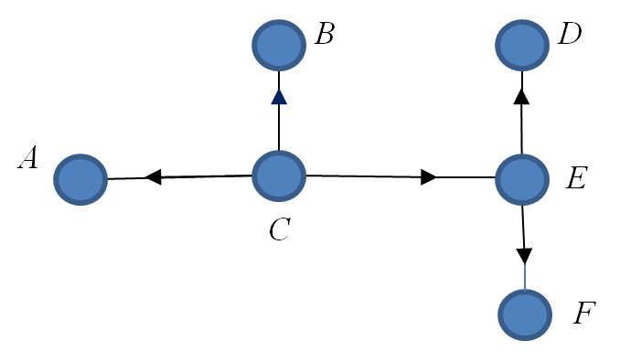
Drawing in the recommended fashion (we do not need the arrows):
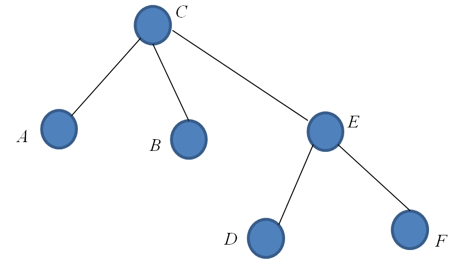
In this example the root is the vertex $C$ and the leaves are the vertices: $A, B, D$, and $F$.
End of Example 31Example 32
The following is a rooted tree. The root is $\text{Bob}$ – which has been indicated by placing the $\text{Bob}$ vertex at the top. The implied orientation for each edge is down.
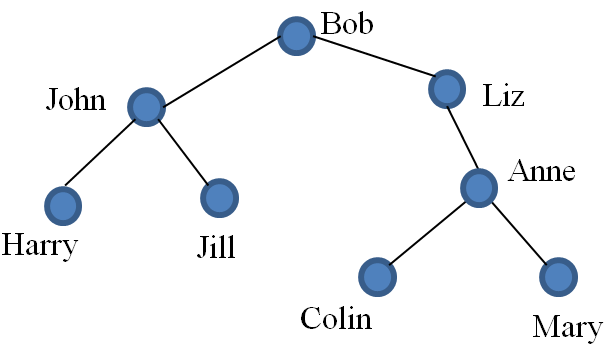
Any tree can be turned into a rooted tree – imagine holding the ‘root’ and letting the tree hang. Note that the choice of root is not unique; it is determined by the application.
If we reconsider Example 32 and make Liz the root we obtain the tree shown below.
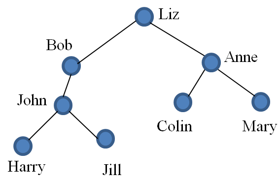
In general however, the root is clearly defined. For example, in a tree representing the management structure of an organisation the root will be the managing director.
A tree is an effective data structure for representing relations between data with a hierarchical element. The classic example is the family tree; but there are many others.
End of Example 3210.3. Tree Properties
The following are some important properties of trees, also refer to Section 3.5.
(i). A tree with $n$ vertices has $n - 1$ edges.
(ii). Every finite connected graph contains a spanning tree (i.e. a subgraph that is a tree), see section 10.4 below.
(iii). Each pair of distinct vertices in a tree is connected by one path.
(iv). The removal of an edge from a tree disconnects the graph.
(v). The addition of an edge to a tree results in a cycle.
(vi). A tree has vertices of degree $1$.
10.4. Spanning Trees
In a problem where the data is represented by a graph it is not unusual that the required solution is a tree that spans the graph. By this we mean a tree that has the same vertices as the graph and uses only the available edges from the graph, i.e. it is a subgraph on all the vertices of the graph.
- A spanning tree for a connected graph $G$ is a connected subgraph on all the vertices of $G$ which is also a tree. One approach for generating a spanning tree involves the following steps:
- Find a cycle in $G$.
- Remove an edge from this cycle.
- Repeat until no cycles remain.
Example 33
Find a spanning tree in the following graph:
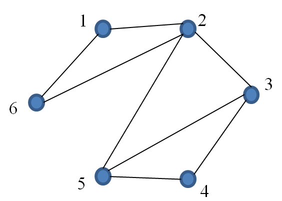
Solution
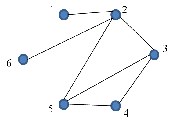
- Choose cycle 1261
- Remove edge $\{ 1, 6 \}$
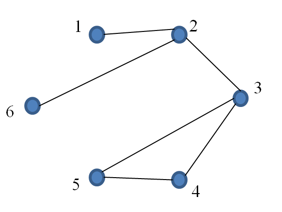
- Choose cycle 2352
- Remove edge $\{ 2, 5 \}$
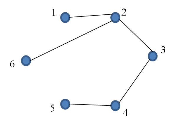
- Choose cycle 3453
- Remove edge $\{ 3, 5 \}$
Note that the solution is not unique as removal of other edges from the cycles generates a different spanning tree. For example, removing edges, $\{ 2, 6 \}$, $\{3, 4 \}$ and $\{ 3, 5 \}$ yields the following:
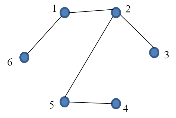
There are other solutions.
End of Example 33Example 34
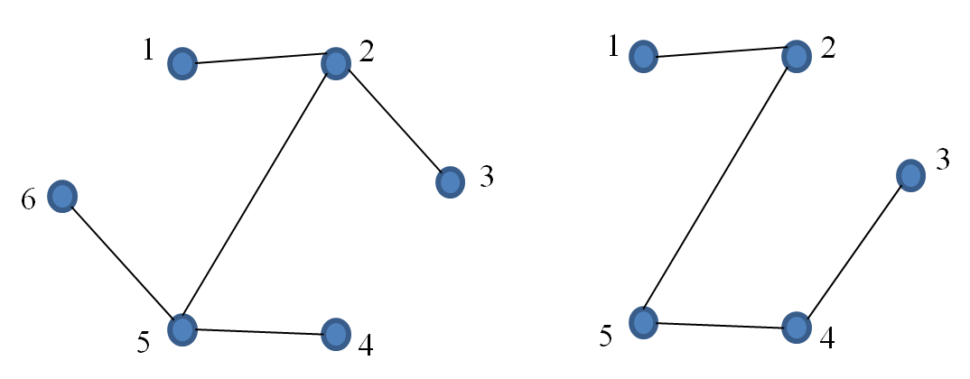
The following two trees are NOT spanning trees for the graph in the previous example. They are both trees but the one on the left is not a subgraph as the original graph does not include the edge $\{ 5, 6 \}$. The one on the right does not span as it does not include the vertex labelled 6.
Note: Recall that a weighted graph is a graph in which the edges have been assigned a weight, i.e. a numerical value. The weight is often used to signify the capacity of what is being modelled by the edge, e.g. bandwidth, max flow rate, etc. In other applications it represents a cost. Many problems revolve around determining a minimum weight spanning tree – a spanning tree in which the sum of the weights along the edges is smaller than for any other spanning tree. There are algorithms for solving this problem, including those by Kruskal and Primm.
End of Example 34 -
11. Searching Trees
Often trees represent data that are related hierarchically and we require some means of searching the tree for a particular item of data. Clearly such a search has to be systematic to ensure that all the vertices are visited. Furthermore, we would also like to ensure that the same vertex is not visited too often. There are two principal algorithms for searching trees: depth first search (DFS) and breadth first search (BFS). The main focus here is on DFS and we present the method supported by examples illustrating pre-order and post-order traversals.
Watch this video:
📹 Binary tree traversal - breadth-first and depth-first strategies
11.1. Depth First Search (DFS)
11.1.1. Depth First Search Algorithm
Depth First Search (DFS) - on a connected graph
(note there are more efficient recursive algorithms for DFS)
0 Make the list empty
1 Choose a start vertex, call it the ‘current vertex’, and label it visited. Add it to the list
2 Repeat
3 If the current vertex has adjacent vertices which are unlabelled then
4 Move to any unlabelled vertex adjacent to the current vertex, label it visited and add it to the list.
Make it the current vertex.
4 Else
5 Delete current vertex from the list and make the last vertex on the list the current vertex.
6 End if
7 Until the list is empty
8 Stop DFS completed.
[ To construct a DFS spanning tree for a graph follow the DFS algorithm but record each new edge that the algorithm uses at step 4. An associated DFS spanning tree is then the vertex set of the subgraph plus the recorded edges ]
In the following two examples we demonstrate operation of the DFS algorithm. The same tree is used in both cases to illustrate the application of DFS in tree traversals where the orderings are different.
Watch this video:
Example 35
Carry out a depth first search of the following rooted tree; the root is at vertex $A$.
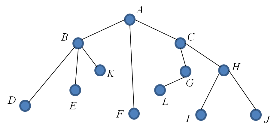
Create a list by going from left to right, starting from the root move down each branch as far as possible before backtracking. Also refer to the section “Further Explanation”.
List
A       ( branch left to vertex B )
AB      ( branch left to vertex D )
ABD 	( vertex D is a dead end, delete it and backtrack to B )
AB      ( branch to vertex E )
ABE 	( vertex E is a dead end, delete it and backtrack to B )
AB      ( branch to vertex K )
ABK     ( vertex K is a dead end, delete it and backtrack to B )
AB      ( vertex B is a dead end, delete it and backtrack to A )
A       ( branch to vertex F )
AF  	( vertex F is a dead end, delete it and backtrack to A )
A       ( branch to vertex C )
AC      ( branch to vertex G )
ACG 	( branch to vertex L )
ACGL 	( vertex L is a dead end, delete it and backtrack to G )
ACG 	( vertex G is a dead end, delete it and backtrack to C )
AC      ( branch to vertex H )
ACH 	( branch to vertex I )
ACHI 	( vertex I is a dead end, delete it and backtrack to H )
ACH 	( branch to vertex J)
ACHJ 	( vertex J is a dead end, delete it and backtrack to H )
ACH 	( vertex H is a dead end, delete it and backtrack to C )
AC      ( vertex C is a dead end and, delete it and backtrack to A )
A       STOP
End of Example 3511.1.2. Pre-ordering
The DFS algorithm can generate different orderings of the search depending on how the visited vertices are recorded. In a pre-ordering the vertices are recorded the FIRST time they are visited (Polish) by the DFS algorithm. In a post-ordering, discussed in Section 11.1.3, a vertex is recorded the LAST time it is visited (reverse Polish) by the DFS algorithm.
Example 36
Depth First Search (DFS) with Pre-order traversal
Carry out a depth first search of the following rooted tree ( root is $A$ ), using pre-ordering to process the vertices.
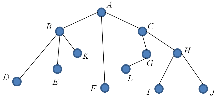
A pre-order traversal of a tree, $T$, starts at the root and then, moving from left to right, traverses each subtree of $T$ in pre-order, continuing until all the vertices have been traversed. A pre-order traversal processes a vertex at the FIRST visit.
The list generated by the DFS in Example 35 is reproduced below in the left-hand column.
Vertices are recorded in the right-hand column, in the “Visited List”, as they are visited.
List Visited List $A$ $( A )$ $AB$ $( AB )$ $ABD$ $( ABD )$ $AB$ $ABE$ $( ABDE )$ $AB$ $ABK$ $( ABDEK )$ $AB$ $A$ $AF$ $( ABDEKF )$ $A$ $AC$ $( ABDEKFC )$ $ACG$ $( ABDEKFCG )$ $ACGL$ $( ABDEKFCGL )$ $ACG$ $AC$ $ACH$ $( ABDEKFCGLH )$ $ACHI$ $( ABDEKFCGLHI )$ $ACH$ $ACHJ$ $( ABDEKFCGLHIJ )$ $ACH$ $AC$ $A$ Hence, for the above tree a pre-order traversal is given by, $ABDEKFCGLHIJ$.
End of Example 36Further Explanation
The following explains the process described above and should be viewed along with the list and the tree. Once a vertex has been “visited” it is added to the “Visited List”. In the description below we define a vertex to be a “dead end” if it is either a leaf (terminal vertex) on a given path, or it is a vertex where its adjacent vertices have all been visited.
First visit the root vertex $A$ and move to its left-most subtree rooted at $B$. After visiting $B$ we move to its left subtree rooted at $D$. This subtree has no other vertices and so we visit $D$ ( $D$ is a dead end ) and backtrack to $B$. From $B$ we move to the subtree rooted at $E$ which has no other vertices and so we visit $E$ ( $E$ is a dead end ) and backtrack to $B$. Next visit the subtree rooted at $K$ which has no other vertices and so we visit $K$ ( $K$ is a dead end ) and backtrack to $B$. All the vertices connected to $B$ have been visited ( $B$ is a dead end ) and so backtrack to $A$. From $A$ move to the subtree rooted at $F$. This subtree has no other vertices and so we visit $F$ ( $F$ is a dead end ) and backtrack to $A$.
Now move from $A$ to the subtree rooted at $C$. After visiting $C$ move to the subtree rooted at $G$. Visit $G$ and move to the subtree rooted at $L$ which has no other vertices and so visit $L$ ( $L$ is a dead end ) and backtrack to $G$, All the vertices connected to $G$ have been visited ( $G$ is a dead end ) and so backtrack to $C$. From $C$ move to the subtree rooted at $H$. After visiting $H$ move to its left subtree rooted at $I$. This subtree has no other vertices and so we visit $I$ ( $I$ is a dead end ) and backtrack to $H$. Next visit the subtree rooted at $J$ which has no other vertices ( $J$ is a dead end ) and so we visit $J$ and backtrack to $H$. All the vertices connected to $H$ have been visited ( $H$ is a dead end ) and so backtrack to $C$. All the vertices connected to $C$ have been visited ( $C$ is a dead end ) and so backtrack to the root $A$ ( $A$ is a dead end ).
11.1.3. Post-Ordering
In the next example we repeat the depth first search but use post-ordering instead.
Example 37
DFS with Post-order traversal
Carry out a depth first search of the following rooted tree ( root is $A$ ), using post-ordering to record the vertices.
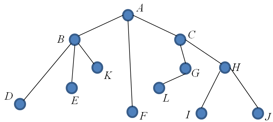
We use the same vertex list generated by the DFS in the previous example on pre-ordering. A post-order traversal of a tree operates from left to right, starting at the root, building as long a path as possible and going left when available. When we reach a leaf ( terminal vertex ) it is visited and we backtrack to its parent. The parent however is not itself visited until all of its descendants have been visited. Referring to the section, “Further Explanation”, this approach corresponds to adding vertices to the Visited List as soon as they are classed as “dead end”.
The list generated by the DFS in Example 35 is reproduced below in the left-hand column.
Vertices are recorded in the right-hand column, in the “Visited List”, as they are visited.
List Visited List $A$ $()$ $AB$ $ABD$ $AB$ $(D)$ $ABE$ $AB$ $(DE)$ $ABK$ $AB$ $(DEK)$ $A$ $(DEKB)$ $AF$ $A$ $( DEKBF )$ $AC$ $ACG$ $ACGL$ $ACG$ $( DEKBFL )$ $AC$ $( DEKBFLG )$ $ACH$ $ACHI$ $ACH$ $( DEKBFLGI )$ $ACHJ$ $ACH$ $( DEKBFLGIJ )$ $AC$ $( DEKBFLGIJH )$ $A$ $( DEKBFLGIJHC ) \\ ( DEKBFLGIJHCA )$ Hence, for the above tree a post-order traversal is given by, $DEKBFLGIJHCA$.
A post-order traversal prints out the content of a vertex when it is LAST visited.
If you compare the two variations on DFS you will see that the order of vertex visits used in the search process is the same on both occasions (look at the evolution on the left hand side of the outputs) even though the sequence of recorded visits are different.
Note that this DFS can, with minor modification, be applied to graphs and digraphs as well but this topic is not covered here.
End of Example 3711.2. Breadth First Search
Breadth First Search (BFS) - on a connected graph
(note there are more efficient recursive algorithms for BFS)
In this algorithm ‘the list’ refers to a list of visited vertices which have not been fully explored.
0 Make the list empty
1 Choose a start vertex, call it the ‘current vertex’, label it visited and add it to the list
2 Repeat
3 If the current vertex has unlabelled vertices adjacent to it then
4 Visit every vertex adjacent to the current vertex and add them to the list.
5 Else
6 Delete the current vertex from the list and make the first vertex on the list the current vertex.
7 End if
8 Until the list is empty.
9 Stop - end of Breadth First Search.
To construct a BFS spanning tree for a graph follow the BFS algorithm but record each new edge that the algorithm uses at step 4. The associated BFS spanning tree is then the vertex set of the graph plus the recorded edges.
A BFS, or breadth first traversal, visits the vertices of a tree level by level, moving from left to right at each level, so that all vertices at the same level are visited before moving down to the next level. This form of traversal is sometimes called a level order traversal.
Watch this video:
Example 38
Carry out a breadth first search of the following rooted tree ( root is $A$ ).
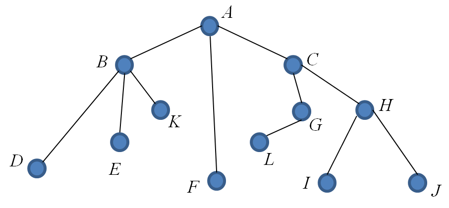
See below for an explanation of how the list is constructed.
List
A
ABFC
BFC
BFCDEK
FCDEK
CDEK
CDEKGH
DEKGH
EKGH
KGH
GH
GHL
HL
HLIJ
LIJ
IJ
J
( )
End of Example 38Construction of Lists
We rewrite the tree so that the levels can easily be identified.
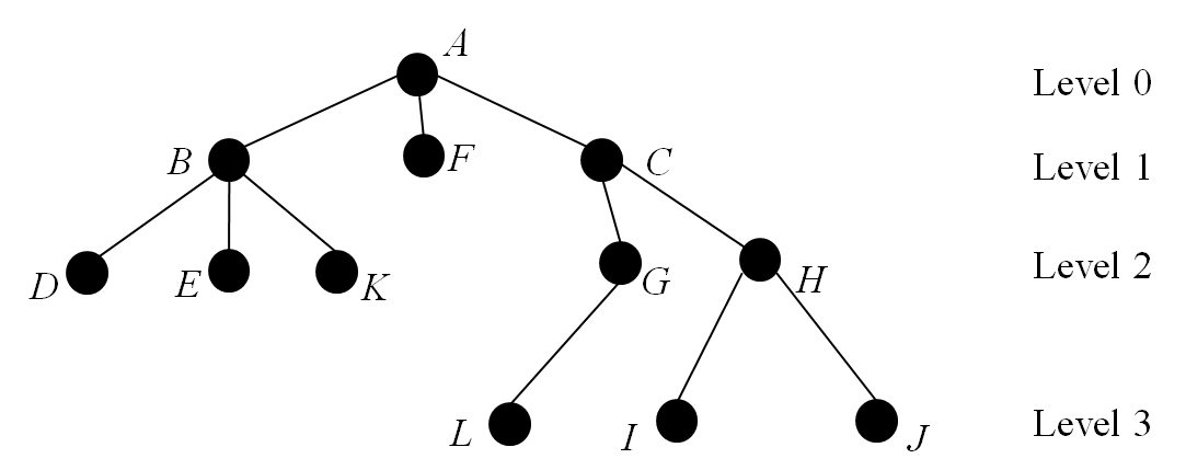
To generate the list given above using a BFS proceed as follows:
- Start at Level 0
- Add vertex $A$ to the list ( $A$ ).
- From left to right add all vertices at Level 1 adjacent to $A$ to the list ($ABFC$ ).
- All vertices at Level 1, adjacent to $A$, have now been added, so remove $A$ from the list ( $BFC$ ). Classify $A$ as visited.
- Move to Level 1
- Add all vertices at Level 2 adjacent to $B$, from left to right, to the list ( $BFCDEK$ ).
- All vertices at Level 2, adjacent to $B$, have been added, so remove $B$ from the list ( $FCDEK$ ).
Classify $B$ as visited. - Move right to $F$. There are no vertices at Level 2 adjacent to $F$, so remove F from the list ( $CDEK$ ).
Classify $F$ as visited. - Move right to $C$. Add all vertices at Level 2, adjacent to $C$, to the list ( $CDEKGH$ ).
- All vertices at Level 2, adjacent to $C$, have been added, so remove $C$ from the list ( $DEKGH$ ).
Classify $C$ as visited.
- Move to Level 2
- At Level 3 there are no vertices adjacent to $D$, so remove $D$ from the list ( $EKGH$ ).
Classify $D$ as visited. - At Level 3 there are no vertices adjacent to $E$, so remove $E$ from the list ( $KGH$ ).
Classify $E$ as visited. - At Level 3 there are no vertices adjacent to $K$, so remove $K$ from the list ( $GH$ ).
Classify $K$ as visited. - Move right to $G$. Add all vertices at Level 3, adjacent to $G$, to the list ( $GHL$ ).
- All vertices at Level 3, adjacent to $G$, have now been added, so remove $G$ from the list ( $HL$ ).
Classify $G$ as visited. - Move right to vertex $H$. Add all vertices at Level 3, adjacent to $H$, to the list ( $HLIJ$ ).
- All vertices at Level 3, adjacent to $H$, have now been added, so remove $H$ from the list ( $LIJ$ ).
Classify $H$ as visited.
- Move to Level 3
- At Level 4 there are no vertices adjacent to $L$ so remove $L$ from the list ( $IJ$ ).
Classify $L$ as visited. - At Level 4 there are no vertices adjacent to $I$ so remove $I$ from the list ( $J$ ).
Classify $I$ as visited. - At Level 4 there are no vertices adjacent to $J$ so remove $J$ from the list.
Classify $J$ as visited. - We are left with the empty list, ( ).
Referring to the diagram and the explanation above, a breadth first search gives the vertex sequence:
$ABFCDEKGHLIJ$, i.e. the vertices are listed in the order they were classed as visited. The process is actually very straightforward in that at each level, moving from left to right, we simply read off all the vertices before moving down the tree to the next level.
Note: The choice of DFS or BFS algorithm is dependent on the problem.
-
Summary
- In this section we have introduced a special type of graph known as a tree which plays an important role in computing and its applications. You should now be able to:
- identify trees from their pictorial representations.
- understand what is meant by the term,” rooted tree”.
- understand what is meant by the term,” spanning tree”.
- find spanning trees for a given graph.
- understand what is meant by the term,” minimum weight spanning tree”.
- understand the depth first search (DFS) and breadth first search (BFS) algorithms for searching trees.
- Carry out a depth first search of a tree using pre-ordering to process the vertices.
- Carry out a depth first search of a tree using post-ordering to process the vertices.
- Carry out a breadth first search of a tree to process the vertices.