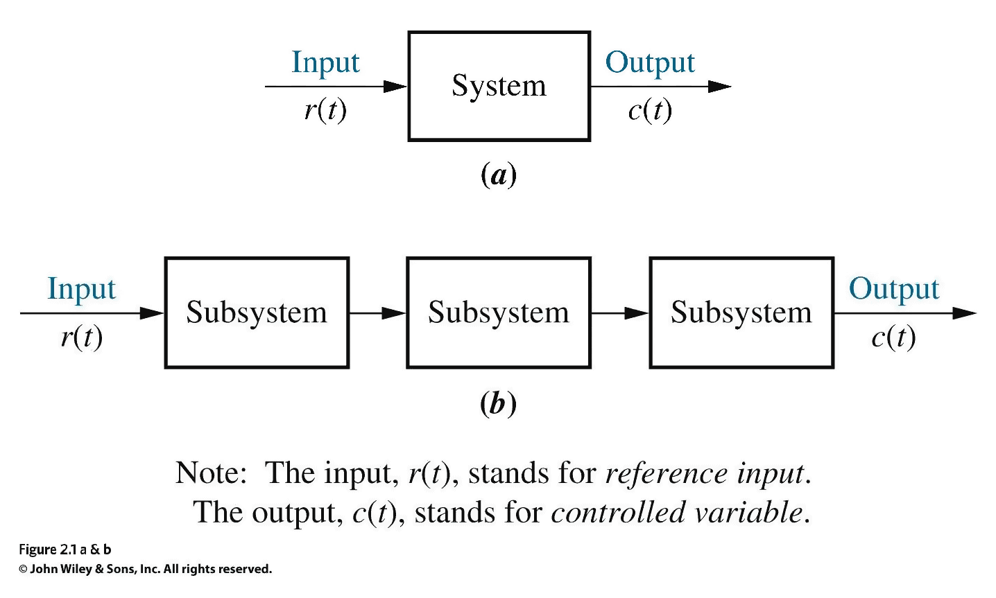
Block One - A
-
10
- Time shift theorem
\begin{align*} \mathcal{L}[f(t - T)] &\rightarrow e^{-s T} F(s) \\ \end{align*} So \begin{align*} g(t) &= f(t - T) &\implies&& G(s) = e^{-s T} F(s) \end{align*}Continues on next tab >
A pure time delay (transport delay) of $T$ seconds can be introduced by multiplying the Laplace transform by $e^{-s T}$.1Chapter 2 - The Laplace transform
- The Laplace transform maps the whole of the time ($t$) domain to the complex $s$-plane \begin{align*} F(s) &= \displaystyle \mathcal{L}[f(t)] &=& \int_0^{\infty} f(t) e^{-st}\,\mathrm{d}t \\ &&&\\\end{align*} and its inverse maps $s$ back to $t$ \begin{align*}f(t) &= \displaystyle \mathcal{L}^{-1}[F(s)] &=& \frac{1}{2\pi j} \int_{\sigma - j \infty}^{\sigma + j \infty} F(s) e^{s t} \mathrm{d}s \end{align*}
9- Linearity theorem
\begin{align*} \mathcal{L}[k f(t)] &\rightarrow k F(s) \\ &\\ \mathcal{L}[f_1(t) + f_2(t)] &\rightarrow F_1(s) + F_2(s) \\ \end{align*} So \begin{align*} g(t) &= k f(t) &\implies&& G(s) = k F(s) \\ &&&&\\ g(t) &= f(t) + h(t) &\implies&& G(s) = F(s) + H(s) \end{align*}
- Time shift theorem
-
12
- Scaling theorem
\begin{align*} \mathcal{L}[f(at)] &\rightarrow \frac{1}{a} F\left(\frac{s}{a}\right) \\ \end{align*} So \begin{align*} g(t) &= f(at) &\implies&& G(s) = \frac{1}{a} F\left(\frac{s}{a}\right) \end{align*}
14- Integration theorem
\begin{align*} \mathcal{L}\left[ \int_0^t f(\tau) \mathrm{d}\tau \right] &= \frac{F(s)}{s} \end{align*}
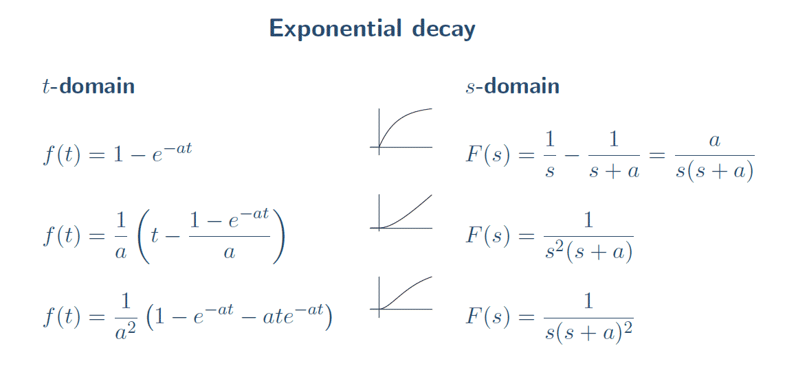
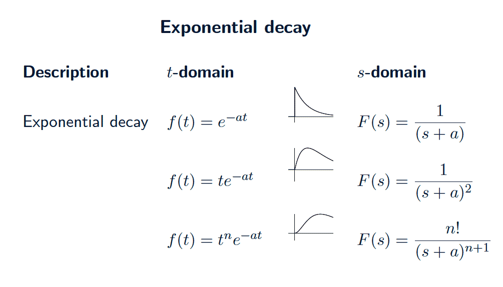
Integration is performed simply by dividing the Laplace transform by $s$.
16- Initial value theorem
\begin{align*} f(0_+) &= \lim_{s \rightarrow \infty} s F(s) \end{align*}
18- MATLAB
Laplace transform of $f(t) = e^{-a t}$ using MATLAB$^1$
syms a t
f = exp(-a*t)
laplace(f)
Inverse Laplace transform of $F(s) = \displaystyle \frac{1}{s+a}$ using MATLAB$^2$
syms a s
F = 1/(s+a)
ilaplace(F)
MATLAB1 MATLAB2
20- Procedure
1. Express $V_c(s)$ as a product of $G(s)$ and $V_0(s)$.
2. Re-write $V_c(s)$ as a sum of simple terms using partial fractions.
3. Manipulate terms algebraically to match entries in a table of Laplace transforms.
4. Obtain inverse Laplace transform of each term using the table.
5. Sum the inverse Laplace transforms.
6. Verify answer.
Continues on next tab >11- Frequency shift theorem
\begin{align*} \mathcal{L}[e^{-a t} f(t)] &\rightarrow F(s+a) \\ \end{align*} So \begin{align*} g(t) &= e^{-a t} f(t) &\implies&& G(s) = F(s+a) \end{align*}
13- Differentiation theorem
\begin{align*} \mathcal{L}\left[ \frac{\mathrm{d}f(t)}{\mathrm{d}t} \right] &= s F(s) - f(0) \\ \mathcal{L}\left[ \frac{\mathrm{d}^2f(t)}{\mathrm{d}t^2} \right] &= s^2 F(s) - s f(0) - \frac{\mathrm{d}f}{\mathrm{d}t}(0) \\ \mathcal{L}\left[ \frac{\mathrm{d}^3f(t)}{\mathrm{d}t^3} \right] &= s^3 F(s) - s^2 f(0) - s \frac{\mathrm{d}f}{\mathrm{d}t}(0) - \frac{\mathrm{d}^2f}{\mathrm{d}t^2}(0) \\ \end{align*}
If the initial conditions are zero, differentiation is performed simply by multiplying the Laplace transform by $s$.
15- Final value theorem
\begin{align*} f(\infty) &= \lim_{s \rightarrow 0} s F(s) \end{align*}
For a unit step input, the final value can be found directly from the transfer function by letting $s \rightarrow 0$
17- Key points, to all of the above
If the initial conditions are zero, differentiation is performed simply by multiplying the Laplace transform by $s$.
Integration is performed simply by dividing the Laplace transform by $s$.
A pure time delay (transport delay) of $T$ seconds can be introduced by multiplying the Laplace transform by $e^{-s T}$.
For a unit step input, the final value can be found directly from the transfer function by letting $s \rightarrow 0$
19Hand calculations
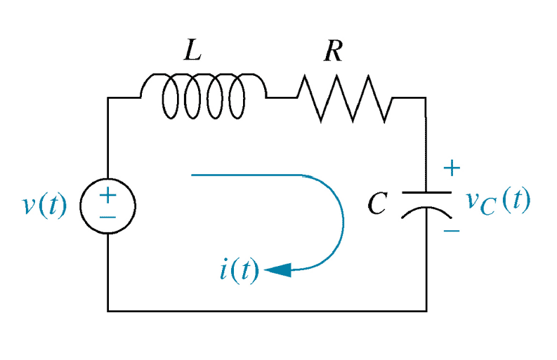
- Example: Second order LRC circuit
\begin{align*} G(s) &= \frac{V_c}{V_{0}}(s) = \frac{1}{L C s^2 + R C s + 1} \end{align*} \begin{align} V_0 && \text{applied EMF} && (\text{volts,} \quad V)\\ V_c && \text{potential difference across capacitor} && (\text{volts,} \quad V)\\ L && \text{inductance} && (\text{henries,} \quad H)\\ R && \text{resistance} && (\text{ohms,} \quad \Omega)\\ C && \text{capacitance} && (\text{farads,} \quad F) \end{align}
An electrical LRC circuit is modelled by transfer function $G(s)$.
For given $L$, $R$ and $C$, find the potential difference across the capacitor $V_c(t)$ in response to a unit step input $V_0(t)$. \begin{align*} V_0(t) &= \begin{cases} 0 {\rm V} & \text{if } t \leq 0 \\ 1 {\rm V} & \text{if } t \gt 0 \end{cases} & V_0(s) &= \frac{1}{s} \end{align*} - Scaling theorem
-
22
- Partial fraction expansion
Factorise $G(s)$, using $s = \frac{-b\pm\sqrt{b^2-4ac}}{2a}$ if necessary, to find the denominators. \begin{align*} s &= \frac{-12\pm\sqrt{12^2-4\times 20}}{2\times 1} & s=-2 \text{or }s=-10 \end{align*} $\qquad \qquad \qquad \text{Hence} $ \begin{align*} V_c(s) &=\frac{20}{s^2 + 12 s + 20} \times \frac{1}{s} \\ &= \frac{20}{s(s+2)(s+10)} \\ &= \frac{A}{s} + \frac{B}{s+2} + \frac{C}{s+10} \end{align*}
Next: all unique linear factors, so find $A, B,$ and $C$ using Heaviside's Quick Cover-Up method.
24- Inverse Laplace transform
Standard transform table has entries for $\displaystyle \frac{1}{s}$ and $\displaystyle \frac{1}{s+a}$ or $\displaystyle \frac{a}{s+a}$. \begin{align*} V_c(s) &=& \frac{1}{s} && -\frac{1.25}{s+2} && +\frac{0.25}{s+10} \\ \\ &=& \frac{1}{s} && -1.25 \times \frac{1}{s+2} && +0.25 \times \frac{1}{s+10} \\ \\ V_c(t) &=& \mathcal{L^-{^1}}{\Bigg[\frac{1}{s}\Bigg]} &&- 1.25 \times \mathcal{L^-{^1}}{\Bigg[\frac{1}{s+2}\Bigg]} &&+ 0.25 \times \mathcal{L^-{^1}}{\Bigg[\frac{1}{s+10}\Bigg]} \end{align*} Next: look up the inverse Laplace transforms.
26- Output
\begin{align*} \large V_c(t) &= \large 1 - 1.25 e^{-2 t} + 0.25 e^{-10 t} \end{align*}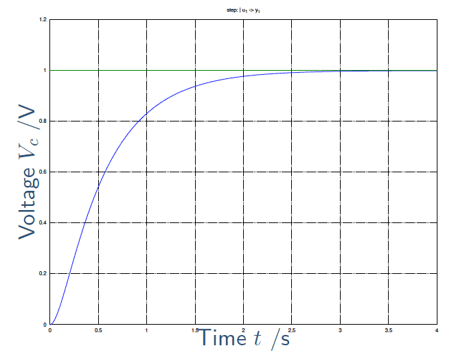
Figure 7
28- Critically-damped: $G(s)$ has repeated real root: $(RC)^2=4LC $
Example: $L=1$ H, $R=20 \Omega$, $C=0.01$ F. % s=-10
\begin{align*} G(s) &= \frac{V_c}{V_{0}}(s) = \frac{1}{L C s^2 + R C s + 1} & V_0(s) &= \frac{1}{s} \end{align*} \begin{align*} V_c(s) &= G(s) \times V_0(s) \\ &= \frac{1}{0.01 s^2 + 0.2 s + 1} \times \frac{1}{s} = \frac{100}{s^2 + 20 s + 100} \times \frac{1}{s} \end{align*}
Next: re-write $V_c$ as a sum of terms using partial fractions.
30- Partial fraction coefficients
Continues on next tab >
\begin{align*} V_c(s) &= \frac{100}{s(s+10)(s+10)} = \frac{A}{s} + \frac{B}{s+10} + \frac{C}{(s+10)^2} \end{align*} Cross-multiplying and equating coefficients of $s^n$ \begin{align*} 100 &= A(s+10)^2 + Bs(s+10) + Cs \\ &= (A+B)s^2 + (20A+10B+C)s + 100A \end{align*} \begin{align*} s^2: && 0 &= A+B &&\implies B = -A\\ s^1: && 0 &= 20A+10B+C &&\implies C = -10A\\ s^0: && 100 &= 100 A && \implies A = 1 \end{align*}
$\qquad \qquad \qquad \text{Hence} $
\begin{align*} A &= 1 & B &= -1 & C &= -10 \end{align*}
21- Over-damped: $G(s)$ has 2 real roots: $(RC)^2 \gt 4LC$
Example: $L=0.5$ H, $R=6 \Omega$, $C=0.1$ F. % s=-2,-10
\begin{align*} G(s) &= \frac{V_c}{V_{0}}(s) = \frac{1}{L C s^2 + R C s + 1} & V_0(s) &= \frac{1}{s} \end{align*} \begin{align*} V_c(s) &= G(s) \times V_0(s) \\ &= \frac{1}{0.05 s^2 + 0.6 s + 1} \times \frac{1}{s} = \frac{20}{s^2 + 12 s + 20} \times \frac{1}{s} \end{align*}
Next: re-write $V_c$ as a sum of terms using partial fractions.
23- Partial fraction coefficients
\begin{align*} V_c(s) =\frac{20}{s(s+2)(s+10)} = \frac{A}{s} + \frac{B}{s+2} + \frac{C}{s+10} \end{align*} Using Heaviside's Quick Cover-Up method \begin{align*} A &= 1 \quad & B &= -\frac{5}{4} = -1.25 \quad & C &= \frac{1}{4} = 0.25 \end{align*} \begin{align*} V_c(s) &= \frac{1}{s} - \frac{1.25}{s+2} + \frac{0.25}{s+10} \end{align*}
Next: manipulate terms to match entries in table of transforms.
25- Inverse Laplace transform
\begin{align*} \mathcal{L^-{^1}}{\Bigg[\frac{1}{s}}\Bigg] &= 1 & \mathcal{L^-{^1}}{\Bigg[\frac{1}{s+a}}\Bigg] &= e^{-at} \end{align*} \begin{align*} V_c(t) &= \mathcal{L^-{^1}}{\Bigg[\frac{1}{s}\Bigg]} &-& 1.25 \times \mathcal{L^-{^1}}{\Bigg[\frac{1}{s+2}\Bigg]} &+& 0.25 \times \mathcal{L^-{^1}}{\Bigg[\frac{1}{s+10}\Bigg]} \\ \\ &= 1 &-& 1.25 \times e^{-2t} &+& 0.25 \times e^{-10t} \end{align*}
Finally, verify! (How?)
27- Verification with MATLAB
L = 0.5; R = 6; C = 0.1;
% visual check
G = tf( 1, [ L*C, R*C, 1 ]);
[y, t] = step(G);
x = 1 - 1.25.*exp(-2*t) + 0.25.*exp(-10*t);
figure(1): plot(t,y); title('Step response');
figure(2); plot(t,x); title('Hand calc');
figure(3); plot(t,y-x); title('Difference')
% symbolic check
syms s
ilaplace(1/(L*C*s^2+R*C*s+1)*(1/s))29- Partial fraction expansion
Factorise $G(s)$, using $s = \frac{-b\pm\sqrt{b^2-4ac}}{2a}$ if necessary, to find the denominators. \begin{align*} s &= -10 \text{(repeated)} \end{align*} \begin{align*} V_c(s) &= \frac{100}{s^2 + 20 s + 100} \times \frac{1}{s} \\ &= \frac{100}{s(s+10)(s+10)} \\ &= \frac{A}{s} + \frac{B}{s+10} + \frac{C}{(s+10)^2} \end{align*}
Next: repeated factors, so cross-multiply and equate coefficients.
- Partial fraction expansion
-
32
- Output
\begin{align*} \large V_c(t) &= \large 1 - e^{-10 t} - 10 t e^{-10 t} \end{align*}
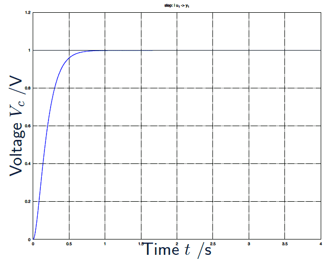
Figure 8
34- Partial fraction expansion
Factorising the quadratic would yield complex roots, so it is better to keep that whole. \begin{align*} V_c(s) &= \frac{10}{s^2+6 s + 10} \times \frac{1}{s} = \frac{A s + B}{s^2 + 6 s + 10} + \frac{C}{s} \end{align*} Cross-multiplying and equating coefficients of $s^n$ \begin{align*} 10 &= (As + B)s + C(s^2+6s+10) \\ &= (A+C) s^2 + (B+6C) s + 10 C \end{align*} \begin{align*} s^2: && 0 &= A+C &&\implies A = -C\\ s^1: && 0 &= B+6C &&\implies B = -6C\\ s^0: && 10 &= 10 C && \implies C = 1 \end{align*} \begin{align*} \therefore A &= -1 & B &= -6 & C &= 1 \end{align*}36- Completing the square
\begin{align*} V_c(s) &= \frac{1}{s} - \frac{s+6}{s^2+6s+10} \\ \end{align*}
\begin{align*} s^2+6s+10 &= \left(s+\frac{6}{2}\right)^2 + \omega^2 \\ &= s^2 + 6s + 9 + \omega^2 &\implies \omega^2 = 1 \\ &= (s+3)^2 + \sqrt{1}^2 \end{align*}
\begin{align*} V_c(s) &= \frac{1}{s} - \frac{s+6}{(s+3)^2+1^2} = \frac{1}{s} - \frac{s+3}{(s+3)^2+1^2} - \frac{3}{(s+3)^2+1^2} \end{align*} Next: inverse transforms.38- Output
\begin{align*} \large V_c(t) &= \large 1 - e^{-3 t} \cos t + 3 \sin t & \;\;\;\large (\zeta = 0.95) \end{align*}
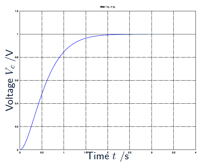
Figure 940- Parameters
Over-damped, $G(S)$ has 2 real roots: $f_v^2 \gt 4mK$Solve by hand and verify in Matlab. Numbers differ, but the method for each case is identical to the electrical examples.
Example: $m=1$ kg, $f_v=3$ N$\cdot$s/m, $K=2$ N/m. % s=-1,-2
Critically-damped, $G(s)$ has repeated real root: $f_v^2=4mK$
Example: $m=1$ kg, $f_v=2$ N$\cdot$s/m, $K=1$ N/m. % s=-1
Under-damped, $G(s)$ has complex pair of roots: $f_v^2 \lt 4mK$
Example: $m=1$ kg, $f_v=2$ N$\cdot$s/m, $K=2$ N/m. % s=-1+/-j31- Inverse Laplace transform
Standard transforms
\begin{align*} \mathcal{L^-{^1}}{\Bigg[\frac{1}{s}\Bigg]} &= 1 & \mathcal{L^-{^1}}{\Bigg[\frac{1}{s+a}\Bigg]} &= e^{-at} & \mathcal{L^-{^1}}{\Bigg[\frac{1}{(s+a)^2}\Bigg]} &= t \times e^{-at} \end{align*} \begin{align*} V_c(s) &= \frac{1}{s} &&- \frac{1}{s+10} &&- \frac{10}{(s+10)^2} \\ \\ &= \frac{1}{s} &&- \frac{1}{s+10} &&- 10 \times \frac{1}{(s+10)^2} \\ V_c(t) &= \mathcal{L^-{^1}}{\Bigg[\frac{1}{s}\Bigg]} &&- \mathcal{L^-{^1}}{\Bigg[\frac{1}{s+10}\Bigg]} &&- 10 \times \mathcal{L^-{^1}}{\Bigg[\frac{1}{(s+10)^2}\Bigg]} \\ \\ &= 1 &&- e^{-10t} &&-10 \times t \times e^{-10t} \end{align*}33Chapter 2 - The Laplace transform
- Under-damped, $G(s)$ has complex pair of roots: $(RC)^2 \lt 4LC$
Example: $L=1$ H, $R=6 \Omega$, $C=0.1$ F. % s=-3+/-j
\begin{align*} G(s) &= \frac{V_c}{V_{0}}(s) = \frac{1}{L C s^2 + R C s + 1} & V_0(s) &= \frac{1}{s} \end{align*}
\begin{align*} V_c(s) &= G(s) \times V_0(s) \\ &= \frac{1}{0.1 s^2 + 0.6 s + 1} \times \frac{1}{s} = \frac{10}{s^2 + 6 s + 10} \times \frac{1}{s} \end{align*}
Next: re-write $V_c$ as a sum of terms using partial fractions.35- Completing the square
Recall the standard inverse transforms. \begin{align*} \mathcal{L^-{^1}}{\Bigg[\frac{s}{s^2+\omega^2}\Bigg]} &= \cos \omega t & \mathcal{L^-{^1}}{\Bigg[\frac{1}{s}\Bigg]} &= 1 \\ \mathcal{L^-{^1}}{\Bigg[\frac{\omega}{s^2+\omega^2}\Bigg]} &= \sin \omega t & \mathcal{L^-{^1} [\mathit{F}(s+a)]} &= e^{-at} \mathcal{L^-{^1}{ [\mathit{F}(s)]}} \end{align*} \begin{align*} V_c(s) &= \frac{1}{s} - \frac{s+6}{s^2+6s+10} \end{align*} The inverse transform of the quadratic term can be found by ''completing the square'' and using the frequency shift theorem.
Next: completing the square37- Inverse Laplace transform
Again recall the standard inverse transforms. \begin{align*} \mathcal{L^-{^1}}{\Bigg[\frac{s}{s^2+\omega^2}\Bigg]} &= \cos \omega t & \mathcal{L^-{^1}}{\Bigg[\frac{1}{s}\Bigg]} &= 1 \\ \mathcal{L^-{^1}}{\Bigg[\frac{\omega}{s^2+\omega^2}\Bigg]} &= \sin \omega t & \mathcal{L^-{^1}}{[F(s+a)]} &= e^{-at} \mathcal{L^-{^1}}{[F(s)]} \end{align*}
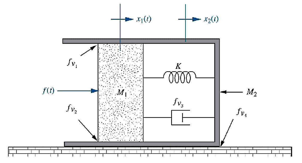
\begin{align*} V_c(s) &=& \frac{1}{s} &- \frac{s+3}{(s+3)^2+1^2} &- 3\times \frac{1}{(s+3)^2+1^2} \\ \\ V_c(t) &=& \mathcal{L^-{^1}}{\Bigg[\frac{1}{s}\Bigg]} &- \mathcal{L^-{^1}}{\Bigg[\frac{s+3}{(s+3)^2+1^2}\Bigg]} &- 3\times\mathcal{L^-{^1}}{\Bigg[\frac{1}{(s+3)^2+1^2}\Bigg]} \\ \\ &=& 1 &- e^{-3t} \cos t &- 3 \times e^{-3t} \sin t \end{align*}39- Example: Second order mechanical system A mechanical mass-damper-spring system is modelled by the transfer function $G(s)$. \begin{align*} G(s) &= \frac{X}{F}(s) = \frac{1}{ms^2 + f_v s + K} \end{align*} $$ \begin{array}{abcde} F & \text{applied force} & \text{(newtons,} & \text{N)} \\ X & \text{displacement} & \text{((metres,} & \text{m)}\\ m & \text{mass} & \text{((kilogrammes,} & \text{kg)}\\ f_v & \text{damping} & \text{((newton-seconds per metre,} & \text{N·s/m))}\\ K & \text{spring stiffness} & \text{((newtons per metre,} & \text{N/m))}\\ \end{array} $$
For given $m$, $f_v$, $K$, find the displacement $X(t)$ in response to a unit step input $F(t)$. \begin{align*} F(t) &= \begin{cases} 0 {\rm N} & \text{if } t \leq 0 \\ 1 {\rm N} & \text{if } t \gt 0 \end{cases} & F(s) &= \frac{1}{s} \end{align*}
- Output
-
42
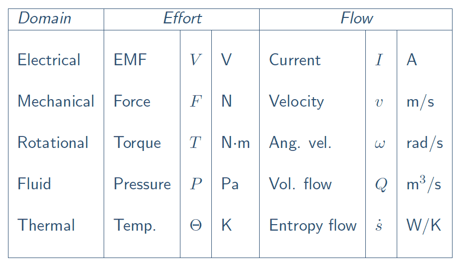
- Physical systems
Physical systems are governed by conservation laws:
Conservation of Energy (including Mass)Conservation of MomentumConservation of Angular MomentumConservation of Electric Charge
41Chapter 2 - Modelling
- Mathematical modelling
1. Determine the equations that govern the individual components
Hooke's Law (springs)Ohm's Law (resistance)Faraday's Law (induction)
2. Determine how the components interact
Newton's Laws (motion)Kirchhoff's Circuit Laws (KCL, KVL)
3. Make approximations and simplifications
LinearisationThévenin's and Mayer-Norton's43- Energetic systems
Power is the universal currency of physical systems.
Intra-domain interaction:Electrical-ElectricalMechanical-Mechanical
Inter-domain interaction:Electrical-Mechanical (Mechatronics)Thermal-Fluid (Thermofluids)
Power must be conserved at all times in each interaction.45Components
- Components
Ideal ElectricalIdeal MechanicalIdeal RotationalIdeal Transformers
47- Constitutive Relations: Electrical
Ideal Inductor\begin{align*} \large I &= \frac{\lambda}{L} & \qquad \frac{\mathrm{d} \lambda}{\mathrm{d}t} &= V \end{align*}
Ideal Resistor\begin{align*} \large V &= I R \end{align*}
Ideal Capacitor\begin{align*} \large V &= \frac{q}{C} & \qquad \large \frac{\mathrm{d}q}{\mathrm{d}t} &= I \end{align*}49- Constitutive Relations: Mechanical
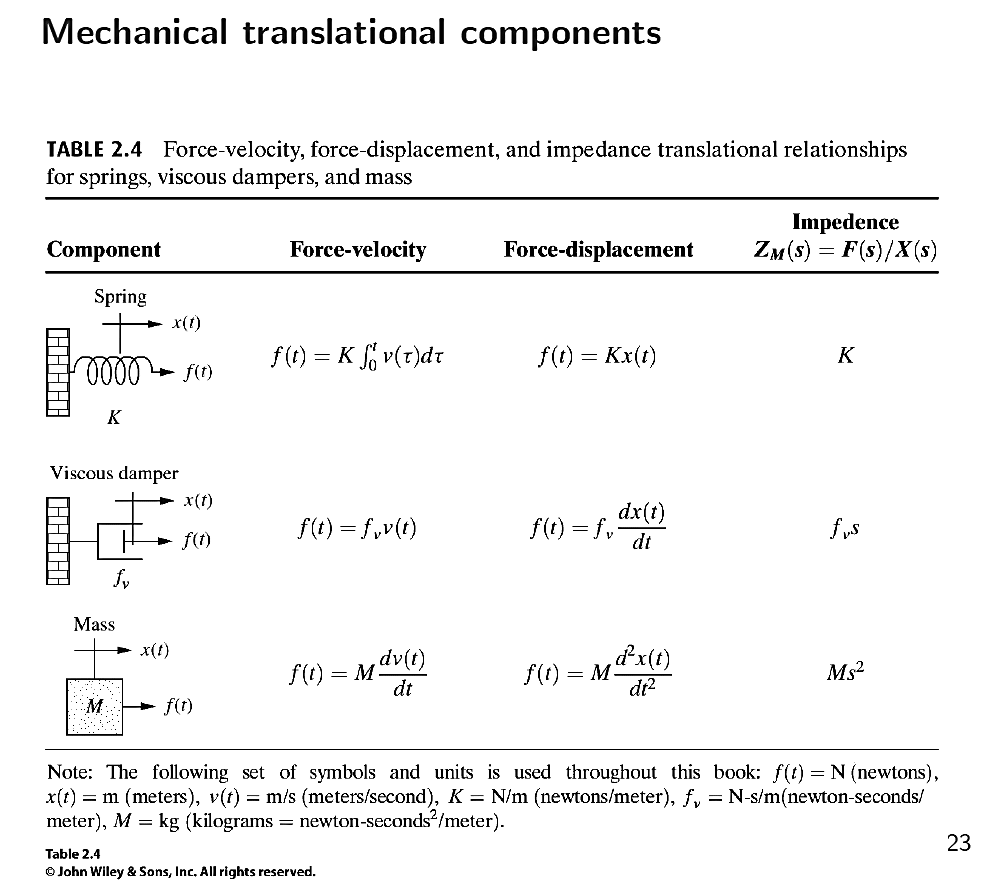
Ideal Mass\begin{align*} \large v &= \frac{p}{m} & \qquad \frac{\mathrm{d}p}{\mathrm{d}t} &= F \end{align*}
Ideal Damper\begin{align*} \large F &= f_v v \end{align*}
Ideal Spring\begin{align*} \large F &= K x & \qquad \frac{\mathrm{d}x}{\mathrm{d}t} &= v \end{align*}
- Physical systems
-
51
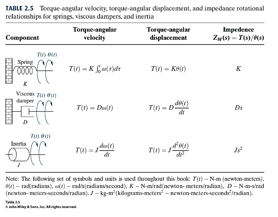
- Constitutive Relations: Rotational
Ideal Inertia\begin{align*} \large \omega &= \frac{p}{J} & \qquad\frac{\mathrm{d}p}{\mathrm{d}t} &= T \end{align*}
Ideal Damper\begin{align*} \large T &= D \omega \end{align*}
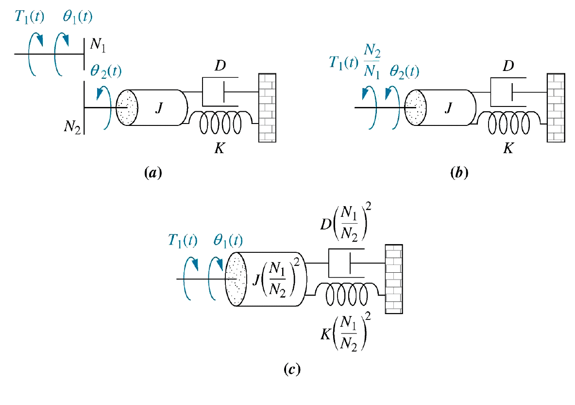
Ideal Spring\begin{align*} \large T &= K \theta & \qquad \frac{\mathrm{d}\theta}{\mathrm{d}t} &= \omega \end{align*}53- Levers
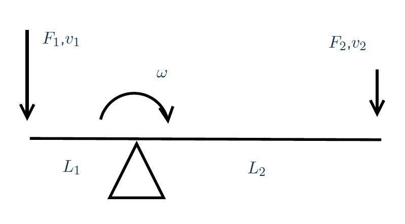
Figure 14
\begin{align*} \large\frac{v_1}{L_1} &= \large\omega = \frac{v_2}{L_2} \end{align*}
\begin{align*} \large\frac{v_1}{v_2} &= \large\frac{L_1}{L_2} \end{align*}55- Constitutive Relations: Motors
Ideal Motor\begin{align*} \large V_1 I_1 &= T_2 \omega_2 & \qquad \frac{T_2}{V_1} &= \large n = \frac{I_1}{\omega_2} \end{align*}
Ideal Cam or Rack & Pinion, etc.\begin{align*} \large T_1 \omega_1 &= \large F_2 v_2 & \qquad \frac{F_2}{T_1} &= n = \frac{\omega_1}{v_2} \end{align*}
57Modelling (Cont.)
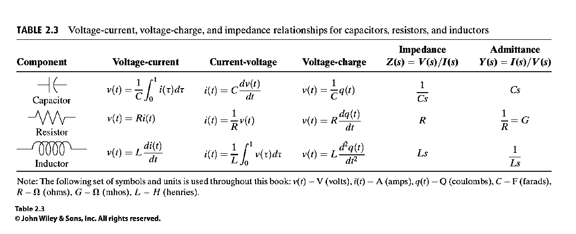
- Impedance and Admittance: Electrical
Ideal Inductor\begin{align*} \large I &= \frac{\lambda}{L} & \qquad \frac{\mathrm{d}\lambda}{\mathrm{d}t} &= V \end{align*}
Ideal Resistor\begin{align*} \large V &= I R \end{align*}
Ideal Capacitor\begin{align*} \large V &= \frac{q}{C} & \qquad \frac{\mathrm{d}p}{\mathrm{d}t} &= I \end{align*}59- Impedance and Admittance: Electrical
Continues on next tab
Ideal Inductor\begin{align*} \large \frac{V}{I} &= L s & \frac{I}{V} &= \frac{1}{L s} \end{align*}
Ideal Resistor\begin{align*} \large \frac{V}{I} &= R & \frac{I}{V} &= \frac{1}{R} \end{align*}
Ideal Capacitor\begin{align*} \large \frac{V}{I} &= \frac{1}{C s} & \frac{I}{V} &= C s \end{align*}
(Nise, p 49 / 47)52Ideal Transformer Components
- Constitutive Relations: Transformers
Ideal Electrical Transformer\begin{align*} \large V_1 I_1 &= V_2 I_2 & \frac{V_2}{V_1} &= n = \frac{I_1}{I_2} & n = \frac{N_2}{N_1} \end{align*}
Ideal Mechanical Lever\begin{align*} \large F_1 v_1 &= F_2 v_2 & \frac{F_2}{F_1} &= n = \frac{v_1}{v_2} & n = \frac{L_1}{L_2} \end{align*}
Ideal Rotational Gear\begin{align*} \large T_1 \omega_1 &= T_2 \omega_2 & \frac{T_2}{T_1} &= n = \frac{\omega_1}{\omega_2} & n = \frac{D_2}{D_1} \end{align*}54- Gears
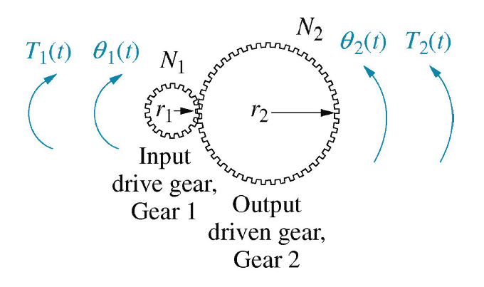
Figure 15
\begin{align*} \large r_1 \omega_1 &= \large v = r_2 \omega_2 \end{align*} \begin{align*} \large \frac{\omega_1}{\omega_2} &= \large \frac{r_2}{r_1} \end{align*}56- Impedance and Admittance
Impedance\begin{align*} \large Z(s) &= \frac{V}{I}(s) & Z_M(s) &= \frac{F}{x}(s) & Z_M(s) &= \frac{T}{\theta}(s) \\ \end{align*}
Admittance\begin{align*} \large Y(s) &=\frac{I}{V}(s) & Y_M(s) &= \frac{x}{F}(s) & Y_M(s) &= \frac{\theta}{T}(s) \\ \end{align*}
58- Impedance and Admittance: Electrical
Ideal Inductor\begin{align*} \large I &= \frac{\lambda}{L} & \qquad s \lambda &= V \end{align*}
Ideal Resistor\begin{align*} \large V &= I R \end{align*}
Ideal Capacitor\begin{align*} \large V &= \frac{q}{C} & \qquad s q &= I \end{align*} - Constitutive Relations: Rotational
-
61
- Impedance and Admittance: Mechanical
Ideal Mass\begin{align*} \large v &= \frac{p}{m} & \qquad s p &= F \end{align*}
Ideal Damper\begin{align*} \large F &= f_v v \end{align*}
Ideal Spring\begin{align*} \large F &= K x & \qquad s x &= v \end{align*}63- Impedance and Admittance: Rotational
Ideal Inertia\begin{align*} \large \omega &= \frac{p}{J} & \qquad \frac{\mathrm{d}p}{\mathrm{d}t} &= T \end{align*}
Ideal Damper\begin{align*} \large T &= D \omega \end{align*}
Ideal Spring\begin{align*} \large T &= K \theta & \qquad \frac{\mathrm{d}\theta}{\mathrm{d}t} &= \omega \end{align*}65- Impedance and Admittance: Rotational
Ideal Inertia\begin{align*} \large \frac{T}{\omega} &= J s & \qquad \large \frac{\omega}{T} &= \frac{1}{J s} \end{align*}
Ideal Damper\begin{align*} \large \frac{T}{\omega} &= D & \qquad \large \frac{\omega}{T} &= \frac{1}{D} \end{align*}
Ideal Spring\begin{align*} \large \frac{T}{\omega} &= \frac{K}{s} & \qquad \large \frac{\omega}{T} &= \frac{s}{K} \end{align*}67- Impedance and Admittance: Translational
Ideal Mass\begin{align*} \large \frac{F}{x} &= m s^2 & \qquad \large \frac{x}{F} &= \frac{1}{m s^2} \end{align*}
Ideal Damper\begin{align*} \large \frac{F}{x} &= f_v s & \qquad \large \frac{x}{F} &= \frac{1}{f_v s} \end{align*}
Ideal Spring\begin{align*} \large \frac{F}{x} &= K & \qquad \large \frac{x}{F} &= \frac{1}{K} \end{align*}60- Impedance and Admittance: Mechanical
Ideal Mass\begin{align*} \large v &= \frac{p}{m} & \frac{\mathrm{d}p}{\mathrm{d}t} &= F \end{align*}
Ideal Damper\begin{align*} \large F &= f_v v \end{align*}
Ideal Spring\begin{align*} \large F &= K x & \frac{\mathrm{d}x}{\mathrm{d}t} &= v \end{align*}62- Impedance and Admittance: Mechanical
Ideal Mass\begin{align*} \large \frac{F}{v} &= m s & \large \frac{v}{F} &= \frac{1}{m s} \end{align*}
Ideal Damper\begin{align*} \large \frac{F}{v} &= f_v & \large \frac{v}{F} &= \frac{1}{f_v} \end{align*}
Ideal Spring\begin{align*} \large \frac{F}{v} &= \frac{K}{s} & \large \frac{v}{F} &= \frac{s}{K} \end{align*}64- Impedance and Admittance: Rotational
Ideal Inertia\begin{align*} \large \omega &= \frac{p}{J} & \qquad s p &= T \end{align*}
Ideal Damper\begin{align*} \large T &= D \omega \end{align*}
Ideal Spring\begin{align*} \large T &= K \theta & \qquad s \theta &= \omega \end{align*}66- Impedance $Z_M$ and Admittance $Y_M$: Electrical
Ideal Inductor\begin{align*} \large \frac{V}{q} &= L s^2 & \qquad \frac{q}{V} &= \frac{1}{L s^2} \end{align*}
Ideal Resistor\begin{align*} \large \frac{V}{q} &= R s & \qquad \frac{q}{V} &= \frac{1}{R s} \end{align*}
Ideal Capacitor\begin{align*} \large \frac{V}{q} &= \frac{1}{C} & \qquad \frac{q}{V} &= C \end{align*}68- Impedance and Admittance: Rotational
Ideal Inertia\begin{align*} \large \frac{T}{\theta} &= J s^2 & \large \qquad \frac{\theta}{T} &= \frac{1}{J s^2} \end{align*}
Ideal Damper\begin{align*} \large \frac{T}{\theta} &= D s & \large \qquad \frac{\theta}{T} &= \frac{1}{D s} \end{align*}
Ideal Spring\begin{align*} \large \frac{T}{\theta} &= K & \large \qquad \frac{\theta}{T} &= \frac{1}{K} \end{align*} - Impedance and Admittance: Mechanical
-
75
- Conservation of power
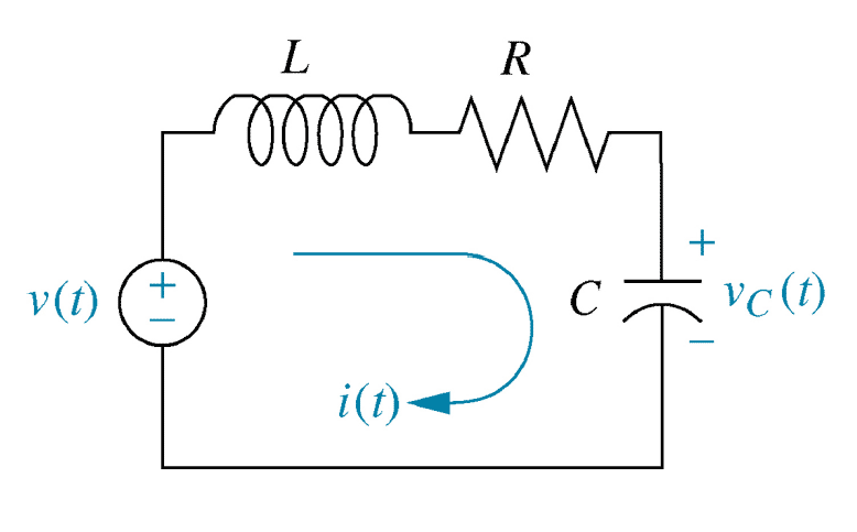 Figure 20
Conservation of power\begin{align*} \large V_L I_L + V_R I_R + V_C I_C &= V_{in} I_{in} \end{align*}77- Kirchhoff’s laws
Kirchhoff's Voltage Law (KVL)The voltages around a closed loop sum to zero.\begin{align*} \large \sum V_{in} - \sum V_{out} &= 0 \end{align*}
Kirchhoff’s Current Law (KCL) The currents at an ideal node sum to zero\begin{align*} \large \sum I_{in} - \sum I_{out} &= 0 \end{align*}
79- Interaction
\begin{align*} \large V_L + V_R + V_C & \large = V_{in} \qquad \qquad \qquad \qquad (KVL) \\ \large \frac{V_L}{I_{in}} + \frac{V_R}{I_{in}} + \frac{V_c}{I_{in}} &= \large \frac{V_{in}}{I_{in}} \\ \large \frac{V_L}{I_L} + \frac{V_R}{I_R} + \frac{V_c}{I_C} &= \large \frac{V_{in}}{I_{in}} \\ \end{align*} \begin{align*} L s + R + \frac{1}{C s} &= \frac{V_{in}}{I_{in}} \\ \frac{I_{in}}{V_{in}} &= \frac{1}{L s + R + \frac{1}{C s}} \\ \frac{I_{in}}{V_{in}} &= \frac{s}{L s^2 + R s + \frac{1}{C}} \\ \end{align*}
74Chapter 2 - Interaction
- Electric circuit
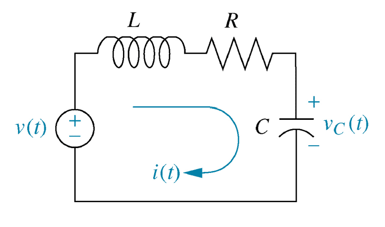 Figure 19
Impedances\begin{align*} \large \frac{V_L}{I_L} &= L s & \qquad \large \frac{V_R}{I_R} &= R & \qquad \large \frac{V_C}{I_C} &= \frac{1}{C s} \end{align*}76Derivation of a Transfer Function from Kirchhoff's voltage law
78- Interaction
Conservation of power\begin{align*} \large V_L I_L + V_R I_R + V_C I_C &= \large V_{in} I_{in} \end{align*}
Kirchhoff’s Laws\begin{align*} \large I_L &= I_R = I_C = I_{in} \qquad\qquad {KCL} \end{align*}
\begin{align*} \large \implies & (V_L + V_R + V_C) I_{in} = V_{in} I_{in} \\ &&\\ \implies I_{in} &= 0 \qquad \text{ or } \\ & V_L + V_R + V_C = V_{in} \qquad\qquad {KVL} \end{align*} - Conservation of power
-
82
- Nodal Analysis
1. Replace all passive components (L,R,C) with their admittances ($Y(s)$).
2. Replace all sources and time variables with their Laplace transforms.
3. Replace transformed voltage sources with transformed current sources.
4. Write Kirchhoff's Current Law at each node.
5. Solve the simultaneous equations for the output.
6. Form the transfer function.
(Nise, pp 54–56 / 51–53)84- Laplace transform of the input
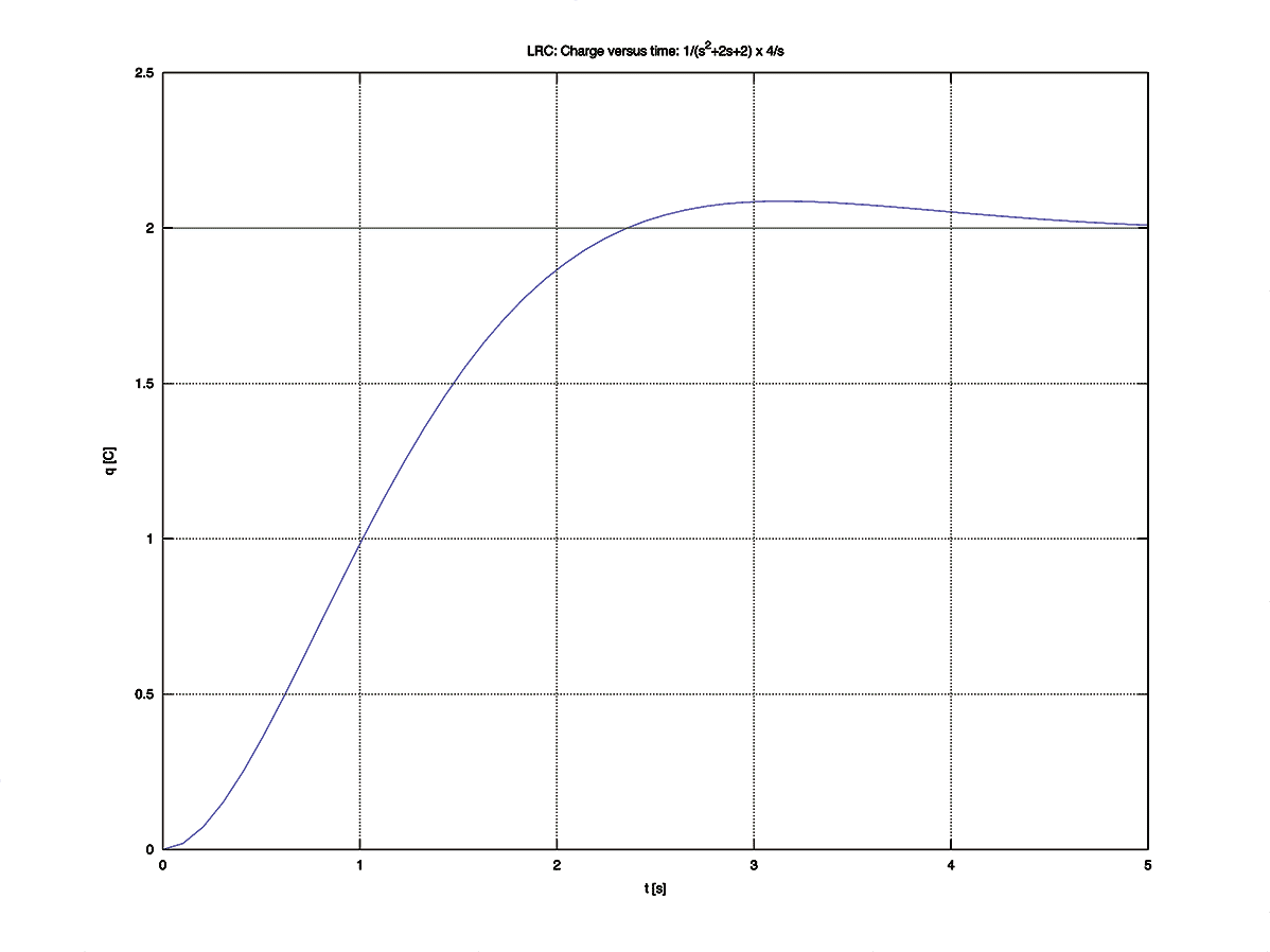
The input is a step of 4 V at time $t = 0$.
From the table of transforms, a unit step is \begin{align*} H(s) &= \frac{1}{s} \end{align*}
Using the linearity theorem, the input is therefore \begin{align*} V(s) &= 4 H(s) = \frac{4}{s} \end{align*} Now find $I(s)$.86- Inverse Laplace transform
\begin{align*} I(s) &= \frac{4}{s^2 + 2 s + 2} \end{align*} Reformat the equation to match the tables of transforms.
Complete the square. \begin{align*} (s+1)^2 = s^2 + 2 s + 1 &\implies& (s+1)^2 + 1 = s^2 + 2s + 2 \end{align*} \begin{align*} \therefore I(s) &= \frac{4}{(s+1)^2 + 1} \end{align*}
Now use the frequency shift theorem.88- Step response
\begin{align*} I(s) &= \frac{4}{s^2 + 2 s + 2} &\qquad \text{c.f. } \frac{k \omega_0^2}{s^2 + 2 \zeta \omega_0 s + \omega_0^2} \\ &&\qquad \omega_0 = \sqrt{2} \qquad \zeta = \frac{1}{\sqrt{2}} \\ &&\\ I(t) &= 4 e^{-t} \sin t \end{align*}
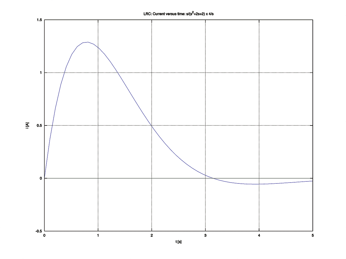 Figure 2281
Mesh and Nodal Analysis
- Mesh Analysis
1. Replace all passive components (L,R,C) with their impedances ($Z(s)$).
2. Replace all sources and time variables with their Laplace transforms.
3. Assume a transform current and current direction in each mesh.
4. Write Kirchhoff's Voltage Law around each mesh.
5. Solve the simultaneous equations for the output.
6. Form the transfer function.
(Nise, pp 51--52 / 49--51)83Example: LRC
- Example: I(t) for LRC using impedences
Find an expression for the current $I(t)$ in a LRC circuit with parameters: \begin{align*} L &= 1 \text{H} & R &= 2 \Omega & C &= 0.5 \text{F} & V(t) &= 4 \text{V if } t \gt 0 \end{align*} Start by finding the Admittance $Y(s)$. \begin{align*} \frac{I}{V}(s) &= \frac{1}{L s + R + \frac{1}{C s}} \\ & \\ &= \frac{s}{L s^2 + R s + \frac{1}{C}} \\ & \\ &= \frac{s}{s^2 + 2 s + 2} \end{align*} Now find $V(s)$.85- I(s)
\begin{align*} I(s) &= \frac{I}{V}(s) \times V(s) \\ &\\ &= \frac{s}{s^2 + 2 s + 2} \times \frac{4}{s} \\ &\\ &= \frac{\require{cancel}\cancel{s}}{s^2 + 2 s + 2} \times \frac{4}{\require{cancel}\cancel{s}} \\ &\\ &= \frac{4}{s^2 + 2 s + 2} \end{align*}
Now find $I(t)$.87- Frequency shift theorem
\begin{align*} I(s) &= \frac{4}{(s+1)^2 + 1} \end{align*} \begin{align*} \text{Let } G(s) &= \frac{1}{s^2+1^2} & \implies & g(t) = \sin t \end{align*} \begin{align*} I(s) &= 4 G(s+1) & \implies & I(t) = 4 e^{-t} g(t) \end{align*}
$$ I(t) = 4 e^{-t} \sin t $$89- Code for plotting $I(t)$ in Matlab or Octave
figure(1)
g_iV = tf([4,0],[1,2,2])
step(g_iV)
title('LRC: Current versus time: s/(s 2+2s+2) x 4/s')
xlabel('t [s]')
ylabel('i [A]')
grid on
Figure 23
print -depsc 'LRC-i.eps'
- Nodal Analysis
-
92
Example: LRC (Cont.)
- Example: Mesh Analysis
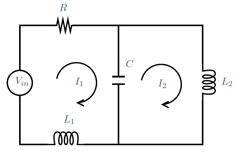 Figure 25
Find an expression for $I_{in}(t)$ given $V_{in}(t)$.94- Collecting terms of $I_1$ and $I_2$
NB: Unverified - check for errors!
Loop 1 \begin{align*} \left(L_1 s + R_1 + \frac{1}{C s}\right) I_1 - \left(\frac{1}{C s}\right) I_2 &= V_{in} \end{align*} Loop 2 \begin{align*} - \left(\frac{1}{C s}\right) I_1 + \left(L_2 s + \frac{1}{C s}\right) I_2 &= 0 \end{align*}
96- Rearrange to form $V_{in}/I_{in}$
NB: Unverified - check for errors! \begin{align*} L_1 s + R + \frac{1}{C s} - \left(\frac{1}{C s}\right) \frac{1}{L_2 C s^2 + 1} &= \frac{V_{in}}{I_{in}} \\ \frac{L_1 s (C s) (L_2 C s^2 +1)}{(C s) (L_2 C s^2 + 1} + \frac{R (C s) (L_2 C s^2 + 1)}{(C s) (L_2 C s^2 + 1)} +& \\ \cdots \frac{(L_2 C s^2 +1)}{(C s) (L_2 C s^2 + 1)} - \left(\frac{1}{C s}\right) \frac{1}{L_2 C s^2 + 1} &= \frac{V_{in}}{I_{in}} \\ \frac{Cs(L_1 L_2 s^3) + Cs(L_1 s) + Cs(L_2 R s^2) + Cs(R) + Cs(L_2 s)}{Cs(C L_2 s^2 + 1)} &= \frac{V_{in}}{I_{in}} \\ \frac{L_1 L_2 s^3 + L_2 R s^2 + (L_1 + L_2) s + R}{C L_2 s^2 + 1} &= \frac{V_{in}}{I_{in}} \\ \frac{C L_2 s^2 + 1}{L_1 L_2 s^3 + L_2 R s^2 + (L_1 + L_2) s + R} &= \frac{I_{in}}{V_{in}} \\ \end{align*}
98Matrices
- Matrices of transfer functions
Structure resulting from a mesh analysis (electrical or mechanical) allows representation in matrix format.
Loop 1 \begin{align*} \left(L_1 s + R_1 + \frac{1}{C s}\right) I_1 - \left(\frac{1}{C s}\right) I_2 &= V_{in} \end{align*} Loop 2 \begin{align*} - \left(\frac{1}{C s}\right) I_1 + \left(L_2 s + \frac{1}{C s}\right) I_2 &= 0 \end{align*}
\begin{align*} \begin{pmatrix} L_1 s + R + \frac{1}{C s} & - \frac{1}{C s} \\ -\frac{1}{C s} & L_2 s + \frac{1}{C s} \end{pmatrix} \begin{pmatrix} I_1 \\ I_2 \end{pmatrix} &= \begin{pmatrix} 1 \\ 0 \end{pmatrix} \begin{pmatrix} V_{in} \end{pmatrix} \end{align*}
100- Outputs
There are a number of outputs we may wish to derive, e.g.
Current through an electrical componentVoltage across an electrical componentForce or torque generated by a mechanical componentTranslational or rotational displacement of a mass
91- Example of using the Frequency Shift theorem
Find $I(t)$ given \begin{align*} I(s) &= \frac{7}{(s+2)^2+9} \end{align*} $\qquad \qquad \qquad \text{Let} $ \begin{align*} G(s) &= \frac{3}{s^2+3^2} &\implies g(t) &= \sin 3 t \end{align*} \begin{align*} I(s) &= \frac{7}{3} G(s+2) \\ I(t) &= \frac{7}{3} e^{-2 t} g(t) \\ &= \frac{7}{3} e^{-2 t} \sin 3 t \end{align*}93- KVL for each loop
NB: Unverified - check for errors!
Loop 1 \begin{align*} R I_1 + \frac{1}{C s}(I_1-I_2) + L_1 s I_1 &= V_{in} \end{align*} Loop 2 \begin{align*} \frac{1}{Cs}(I_2-I_1) + L_2 s I_2 &= 0 \end{align*}
95- Eliminate $I_2$
NB: Unverified - check for errors!
From Loop 2 \begin{align*} \left(L_2 s + \frac{1}{C s}\right) I_2 &= \frac{1}{C s} I_1 \\ I_2 &= \frac{\frac{1}{C s} I_1}{L_2 s + \frac{1}{C s}} \\ I_2 &= \frac{I_1}{L_2 C s^2 + 1} \end{align*} Substitute for $I_2$ in Loop 1 \begin{align*} \left(L_1 s + R + \frac{1}{C s}\right) I_1 - \left(\frac{1}{C s}\right) \frac{I_1}{L_2 C s^2 + 1} &= V_{in} \end{align*}
97- Finally get the current $I_{in}$
\begin{align*} I_{in}(s) &= \frac{I_{in}}{V_{in}}(s) \times V_{in}(s) \\ &= \frac{C L_2 s^2 + 1}{L_1 L_2 s^3 + L_2 R s^2 + (L_1 + L_2) s + R} \times V_{in}(s) \end{align*}
99- Cramer’s rule
\begin{align*} \frac{I_1}{V_{in}}(s) &= \frac{ \left| \begin{matrix} 1 & -\frac{1}{C s} \\ 0 & L_2 s + \frac{1}{C s} \end{matrix} \right| } { \left| \begin{matrix} L_1 s + R + \frac{1}{C s} & - \frac{1}{C s} \\ -\frac{1}{C s} & L_2 s + \frac{1}{C s} \end{matrix} \right| } \end{align*} \begin{align*} \frac{I_2}{V_{in}}(s) &= \frac{ \left| \begin{matrix} L_1 s + R + \frac{1}{C s} & 1 \\ -\frac{1}{C s} & 0 \end{matrix} \right| } { \left| \begin{matrix} L_1 s + R + \frac{1}{C s} & - \frac{1}{C s} \\ -\frac{1}{C s} & L_2 s + \frac{1}{C s} \end{matrix} \right| } \end{align*}
- Example: Mesh Analysis
-
102
- Voltage across a component
Voltage across an electrical component can be obtained by finding the product of its impedance and current.
For an electrical component in loop 1 that is not shared with any other loop,
$\; V_{component} = Z_{component} \times I_1$
$\Large \frac{V_{component}}{V_i} \normalsize = Z_{component} \times \Large \frac{I_1}{V_i}$
For an electrical component shared between loop 1 and loop 2,
$\; V_{component} = Z_{component} \times (I_1 - I_2)$
$\Large \frac{V_{component}}{V_i} \normalsize = Z_{component} \times \Large \frac{I_1 - I_2}{V_i} \normalsize = Z_{component} \times \begin{pmatrix} \Large \frac{I_1}{V_i} - \frac{I_2}{V_i} \end{pmatrix} $
104- Force or torque in a mechanical component
The force generated by a mechanical component can be obtained from the product of its impedance and the displacement of the masses to which it is connected.
For a spring or damper connected to mass 1 only,
$\Large \frac{F_{component}}{F_i} \normalsize = Z_{m,component} \times \Large \frac{X_1}{F_i}$
$\Large \frac{T_{component}}{T_i} \normalsize = Z_{m,component} \times \Large \frac{\theta_1}{T_i}$
For a spring or damper connected to mass 1 and mass 2,
$\Large \frac{F_{component}}{F_i} \normalsize = Z_{m,component} \times \Large \frac{X_1 - X_2}{F_i} \normalsize = Z_{m,component} \times \begin{pmatrix} \Large \frac{X_1}{F_i} - \frac{X_2}{F_i} \end{pmatrix}$
$\Large \frac{T_{component}}{T_i} \normalsize = Z_{m,component} \times \Large \frac{\theta_1 - \theta_2}{T_i} \normalsize = Z_{m,component} \times \begin{pmatrix} \Large \frac{\theta_1}{T_i} - \frac{\theta_2}{T_i} \end{pmatrix}$106- Virtual mass
Where a component is not connected to any mass (like the spring below), a symbolic virtual mass can be used with $m=0$.
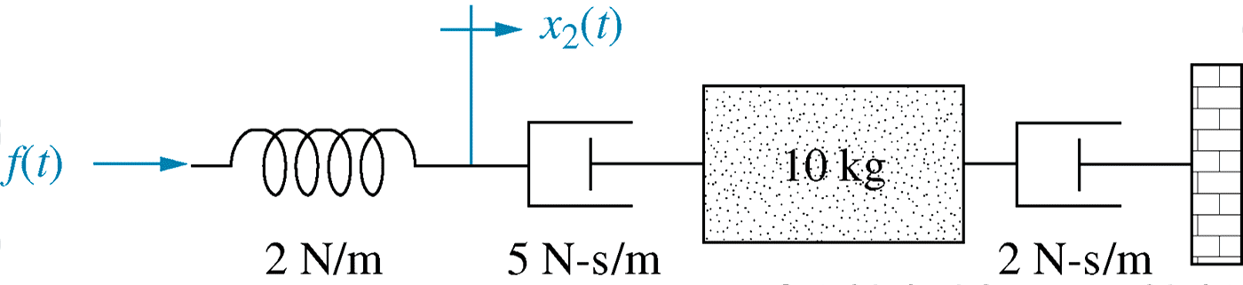 Figure 26
This effectively incorporates Newton's III law into the technique of modelling by inspection (mechanical ``mesh'' analysis).
101- Current through a component
Current through an electrical component can be obtained from the Admittances of each loop to which it is connected.
For an electrical component in loop 1 that is not shared with any other loop,
$\; I_{component} = I_1$
$\Large \frac{I_{component}}{V_i} \normalsize = \Large \frac{I_1}{V_i}$
For an electrical component shared between loop 1 and loop 2,
$\; I_{component} = I_1 - I_2$
$\Large \frac{I_{component}}{V_i} = \frac{I_1 - I_2}{V_i} \normalsize = \Large \frac{I_1}{V_i} - \frac{I_2}{V_i} $
103- Displacement of a mass
The transfer function describing the translational or rotational displacement of a mass due to an applied force or torque is obtained directly from the mathematical model using Cramer’s rule.105- Using the definition of impedance
\begin{align*} Z &= \frac{V}{I} & Z_m &= \frac{F}{X} & Z_m &= \frac{T}{\theta} \\\\ V &= Z \times I & F &= Z_m \times X & T &= Z_m \times \theta \\\\ \frac{V}{V_i} &= Z \times \frac{I}{V_i} & F &= Z_m \times \frac{X}{F_i} & T &= Z_m \times \frac{\theta}{T_i} \\ \end{align*}
109Summary.
- Voltage across a component