Block One - B
-

Chapter 3 - Modelling in the time domain
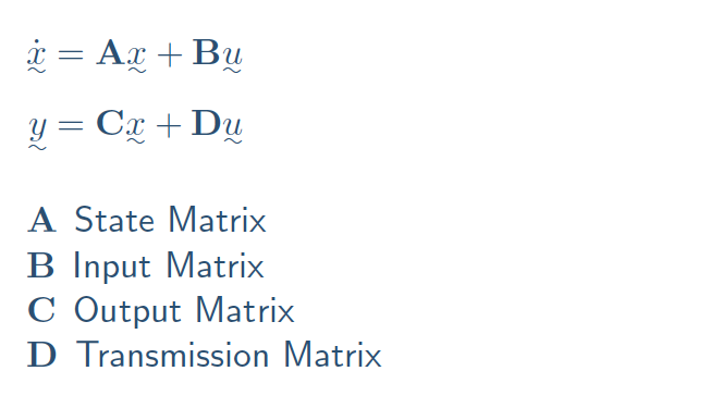
- the general state space representation *
- applying the state space representation *
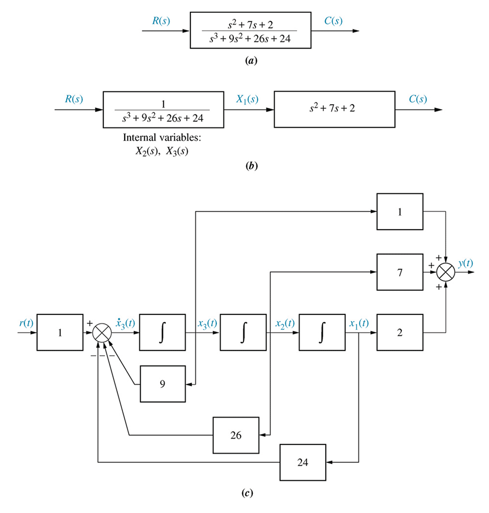
- converting a transfer function to state space *
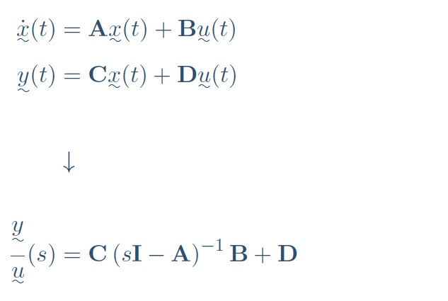
- converting from state space to a transfer function *
- linearisation
Decomposition of a higher a set of first order ODEs.
Conversion of a transfer function into state space (matrix) form.
-
2
- LRC circuit representations
\begin{align*} \text{Second Order ODE} \begin{cases}\;\; L \ddot q + R \dot q + \displaystyle \frac{q}{C} &= V(t) \end{cases} \\ \downarrow &\\ (\text{Using } I = \dot q)\\ \downarrow &\\ L \dot I + R I + \frac{q}{C} = V(t) & \\ \downarrow &\\ \text{2 First Order ODES} \begin{cases} \;\; \dot q &= I \\ \;\; \dot I &= \displaystyle \frac{1}{L} \left( V(t) - \displaystyle \frac{q}{C} -R I \right) \end{cases} \end{align*}
4- Mass Spring Damper representations
\begin{align*} \text{Second Order ODE} \begin{cases}\;\; m \ddot x + f_v \dot x + K x &= F(t) \end{cases} \\ \downarrow &\\ (\text{Using } v = \dot x)\\ \downarrow &\\ m \dot v + f_v v + K x = F(t) & \\ \downarrow &\\ \text{2 First Order ODES} \begin{cases} \;\; \dot x &= v \\ \;\; \dot v &= \displaystyle \frac{1}{m} \left( F(t) - K x - f_v v \right) \end{cases} \end{align*}
6- Decomposition to first order
\begin{align*} a_4 s^4 \theta + a_3 s^3 \theta + a_2 s^2 \theta + a_1 s \theta + a_0 \theta &= u_1(s) \\ a_4 \ddddot \theta ~+~ a_3 \dddot \theta ~+~ a_2 \ddot \theta ~+~ a_1 \dot \theta + a_0 \theta &= u_1(t) \end{align*} \begin{align*} \textrm{Let}\\\\ x_1 &= \theta \\ x_2 &= \dot \theta = \dot x_1 & \implies && \dot x_1 = x_2 \\ x_3 &= \ddot \theta = \dot x_2 & \implies && \dot x_2 = x_3 \\ x_4 &= \dddot \theta = \dot x_3 & \implies && \dot x_3 = x_4 \end{align*}
\begin{align*} a_4 \dot x_4 + a_3 x_4 + a_2 x_3 + a_1 x_2 + a_0 x_1 &= u_1(t) \end{align*}
\begin{align*} \dot x_4 &= \frac{u_1 - a_3 x_4 - a_2 x_3 - a_1 x_2 - a_0 x_1}{a_4} \end{align*}8- General First Order ODEs
Click here to see full equationGeneral First Order ODEs
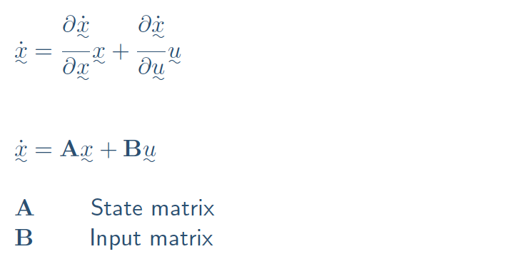
General First Order ODEs \begin{align*} \dot x_1 &= \frac{\partial \dot x_1}{\partial x_1} x_1 + \frac{\partial \dot x_1}{\partial x_2} x_2 + \cdots & + \frac{\partial \dot x_1}{\partial u_1} u_1 + \frac{\partial \dot x_1}{\partial u_2} u_2 + \cdots \\ \dot x_2 &= \frac{\partial \dot x_2}{\partial x_1} x_1 + \frac{\partial \dot x_2}{\partial x_2} x_2 + \cdots & + \frac{\partial \dot x_2}{\partial u_1} u_1 + \frac{\partial \dot x_2}{\partial u_2} u_2 + \cdots \\ &\vdots \\ %y_1 &= \frac{\partial y_1}{\partial x_1} x_1 + \frac{\partial y_1}{\partial x_2} x_2 + \cdots %& + \frac{\partial y_1}{\partial u_1} u_1 + \frac{\partial y_1}{\partial u_2} u_2 + \cdots \\ %y_2 &= \frac{\partial y_2}{\partial x_1} x_1 + \frac{\partial y_2}{\partial x_2} x_2 + \cdots % & + \frac{\partial y_2}{\partial u_1} u_1 + \frac{\partial y_2}{\partial u_2} u_2 + \cdots \\ \end{align*} \begin{align*} \begin{pmatrix} \dot x_1 \\ \dot x_2 \\ \vdots \end{pmatrix} &= \begin{pmatrix} \frac{\partial \dot x_1}{\partial x_1} & \frac{\partial \dot x_1}{\partial x_2} & \cdots \\ \frac{\partial \dot x_2}{\partial x_1} & \frac{\partial \dot x_2}{\partial x_2} & \cdots \\ \vdots & \vdots & \\ \end{pmatrix} \begin{pmatrix} x_1 \\ x_2 \\ \vdots \end{pmatrix} + \begin{pmatrix} \frac{\partial \dot x_1}{\partial u_1} & \frac{\partial \dot x_1}{\partial u_2} & \cdots \\ \frac{\partial \dot x_2}{\partial u_1} & \frac{\partial \dot x_2}{\partial u_2} & \cdots \\ \vdots & \vdots & \\ \end{pmatrix} \begin{pmatrix} u_1 \\ u_2 \\ \vdots \end{pmatrix} % \\ \end{align*}
\begin{align*} \dot x_1 &= \frac{\partial \dot x_1}{\partial x_1} x_1 + \frac{\partial \dot x_1}{\partial x_2} x_2 + \cdots & + \frac{\partial \dot x_1}{\partial u_1} u_1 + \frac{\partial \dot x_1}{\partial u_2} u_2 + \cdots \\ \dot x_2 &= \frac{\partial \dot x_2}{\partial x_1} x_1 + \frac{\partial \dot x_2}{\partial x_2} x_2 + \cdots & + \frac{\partial \dot x_2}{\partial u_1} u_1 + \frac{\partial \dot x_2}{\partial u_2} u_2 + \cdots \\ &\vdots \\ %y_1 &= \frac{\partial y_1}{\partial x_1} x_1 + \frac{\partial y_1}{\partial x_2} x_2 + \cdots %& + \frac{\partial y_1}{\partial u_1} u_1 + \frac{\partial y_1}{\partial u_2} u_2 + \cdots \\ %y_2 &= \frac{\partial y_2}{\partial x_1} x_1 + \frac{\partial y_2}{\partial x_2} x_2 + \cdots % & + \frac{\partial y_2}{\partial u_1} u_1 + \frac{\partial y_2}{\partial u_2} u_2 + \cdots \\ \end{align*} \begin{align*} \begin{pmatrix} \dot x_1 \\ \dot x_2 \\ \vdots \end{pmatrix} &= \begin{pmatrix} \frac{\partial \dot x_1}{\partial x_1} & \frac{\partial \dot x_1}{\partial x_2} & \cdots \\ \frac{\partial \dot x_2}{\partial x_1} & \frac{\partial \dot x_2}{\partial x_2} & \cdots \\ \vdots & \vdots & \\ \end{pmatrix} \begin{pmatrix} x_1 \\ x_2 \\ \vdots \end{pmatrix} + \begin{pmatrix} \frac{\partial \dot x_1}{\partial u_1} & \frac{\partial \dot x_1}{\partial u_2} & \cdots \\ \frac{\partial \dot x_2}{\partial u_1} & \frac{\partial \dot x_2}{\partial u_2} & \cdots \\ \vdots & \vdots & \\ \end{pmatrix} \begin{pmatrix} u_1 \\ u_2 \\ \vdots \end{pmatrix} % \\ \end{align*}
1- LRC circuit representations
\begin{align*} Z(s) &= \frac{V}{I}(s) = L s + R + \frac{1}{C s} \end{align*} \begin{align*} L \dot I + R I + \int \displaystyle \frac{I}{C} {\mathrm d}t &= V(t) \\ &\\ L \ddot q + R \dot q + \displaystyle \frac{q}{C} &= V(t) \end{align*}
3- Mass Spring Damper representations
\begin{align*} Z(s) &= \frac{F}{x}(s) = m s^2 + f_v s + K \end{align*} \begin{align*} m \ddot x + f_v \dot x + K x &= F(t) \end{align*}
5- General 4th order system
A system is defined in the $s$ domain by the transfer function
\begin{align*} \frac{\theta}{u_1}(s) &= \frac{1}{ a_4 s^4 + a_3 s^3 + a_2 s^2 + a_1 s + a_0} \end{align*}
Convert it into a set of 4 first order ODEs and hence represent it in matrix form.
7- Matrix representation
\begin{align*} \begin{matrix} \dot x_1 &=& 0 x_1 &+ 1 x_2 &+ 0 x_3 &+ 0 x_4 &+ 0 u_1 \\ \dot x_2 &=& 0 x_1 &+ 0 x_2 &+ 1 x_3 &+ 0 x_4 &+ 0 u_1 \\ \dot x_3 &=& 0 x_1 &+ 0 x_2 &+ 0 x_3 &+ 1 x_4 &+ 0 u_1 \\ \dot x_4 &=& \frac{-a_0}{a_4} x_1 &+ \frac{-a_1}{a_4} x_2 &+ \frac{-a_2}{a_4} x_3 &+ \frac{-a_3}{a_4} x_4 &+ \frac{1}{a_4} u_1 \end{matrix} \end{align*}
\begin{align*} \begin{pmatrix} \dot x_1 \\ \dot x_2 \\ \dot x_3 \\ \dot x_4 \end{pmatrix} &= \begin{pmatrix} 0 & 1 & 0 & 0 \\ 0 & 0 & 1 & 0 \\ 0 & 0 & 0 & 1 \\ -\frac{a_0}{a_4} & -\frac{a_1}{a_4} & -\frac{a_2}{a_4} & -\frac{a_3}{a_4} \end{pmatrix} \begin{pmatrix} x_1 \\ x_2 \\ x_3 \\ x_4 \end{pmatrix} + \begin{pmatrix} 0 \\ 0 \\ 0 \\ \frac{1}{a_4} \end{pmatrix} u_1 \end{align*}
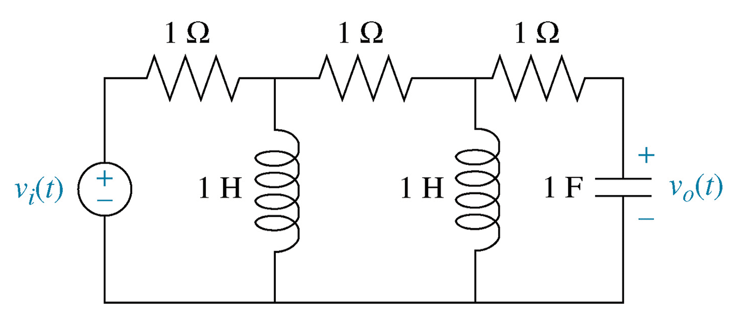
- LRC circuit representations
-
12
- tf2ss
Create a transfer function to represent a system $G(s)$, convert it to state space and compare the responses to a unit step input using $\text {MATLAB} ^1.$
$G(s) = \large \frac{1}{2 s^2 + 3 s + 4}$
num = 1
den = [2, 3, 4]
G1 = tf(num, den)
G2 = ss(G1);
[A,B,C,D] = tf2ss(num, den)
G3 = ss(A,B,C,D);
figure(1); step(G1)
figure(2); step(G2)
figure(3); step(G3)
MATLAB118- Eigenvalues and eigenvectors
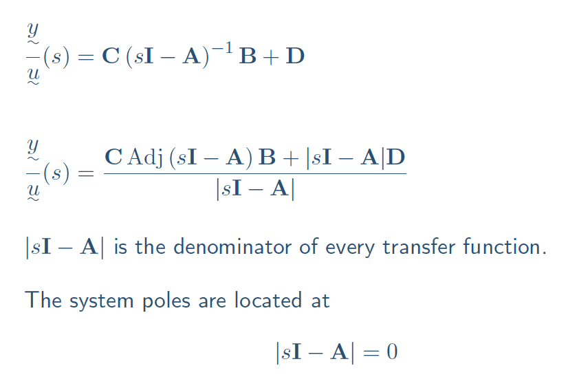
Note the similarity of form of the characteristic equation \begin{align*} | s \mathrm{I} - \mathrm{A} | &= 0 \qquad\qquad\qquad\qquad\qquad\qquad \end{align*}
and eigenvalue formulation \begin{align*} \mathrm{A}\underset{\sim}{x} &= \lambda \underset{\sim}{x} \\ (\lambda \mathrm{I} - \mathrm{A}) \underset{\sim}{x} &= 0 \\ \implies & \underset{\sim}{x} = 0 \qquad \text{ or} \qquad |\lambda \mathrm{I} - \mathrm{A}| = 0 \end{align*} Poles in Matlab: eig(A)
Chapter 3 Summary
- Listen to the summary in the voiceover.
13
Conversion of a State Space Representation into a Transfer Function (SISO) or Transfer Functions (MIMO).
19- ss2tf
Create a state space system $A,B,C,D$ and convert to transfer function form $G(s)$ using $\text {MATLAB} ^2.$
\begin{align*} \mathrm{A} &= \begin{pmatrix}~0,~1\\-2,-3\end{pmatrix} & \mathrm{B} &= \begin{pmatrix}~0,~1\\~5,~0\end{pmatrix}\\ \mathrm{C} &= \begin{pmatrix}~1,~0\\~0,~1\end{pmatrix} & \mathrm{D} &= \begin{pmatrix}~0,~0\\~0,~0\end{pmatrix} \qquad\qquad\qquad\qquad \end{align*}
A = [ 0, 1; -2, -3 ]
B = [ 0, 1; 5, 0 ]
C = eye(2);
D = zeros(2,2)
G = ss(A,B,C,D)
[numU1, denU1] = ss2tf(A, B, C, D, 1)
[numU2, denU2] = ss2tf(A, B, C, D, 2)
MATLAB2
- tf2ss
-
23
- Decomposition
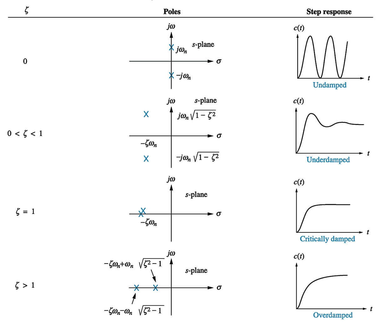
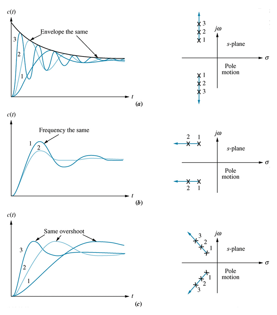
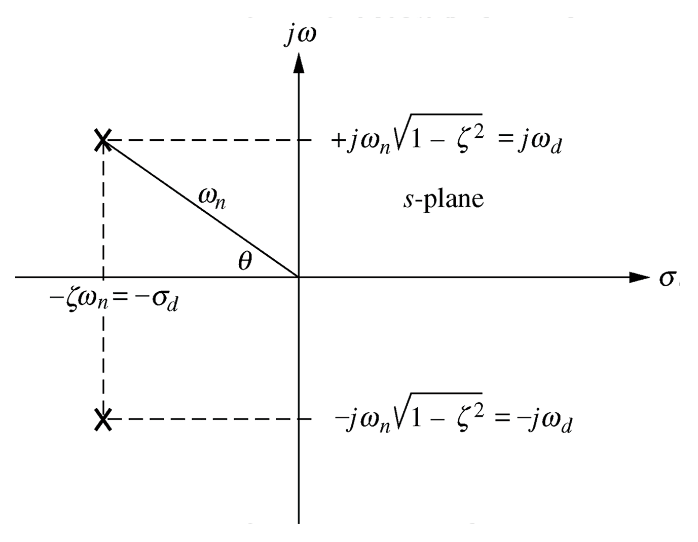
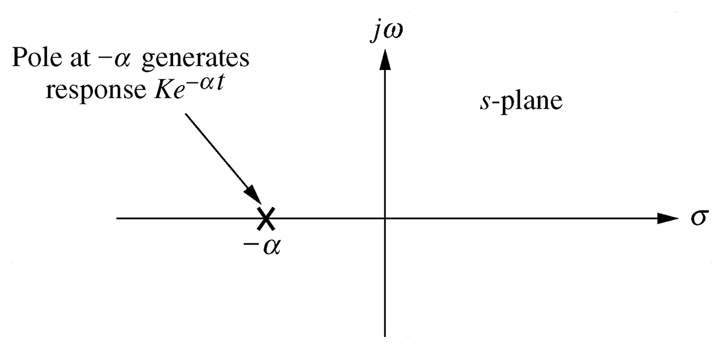
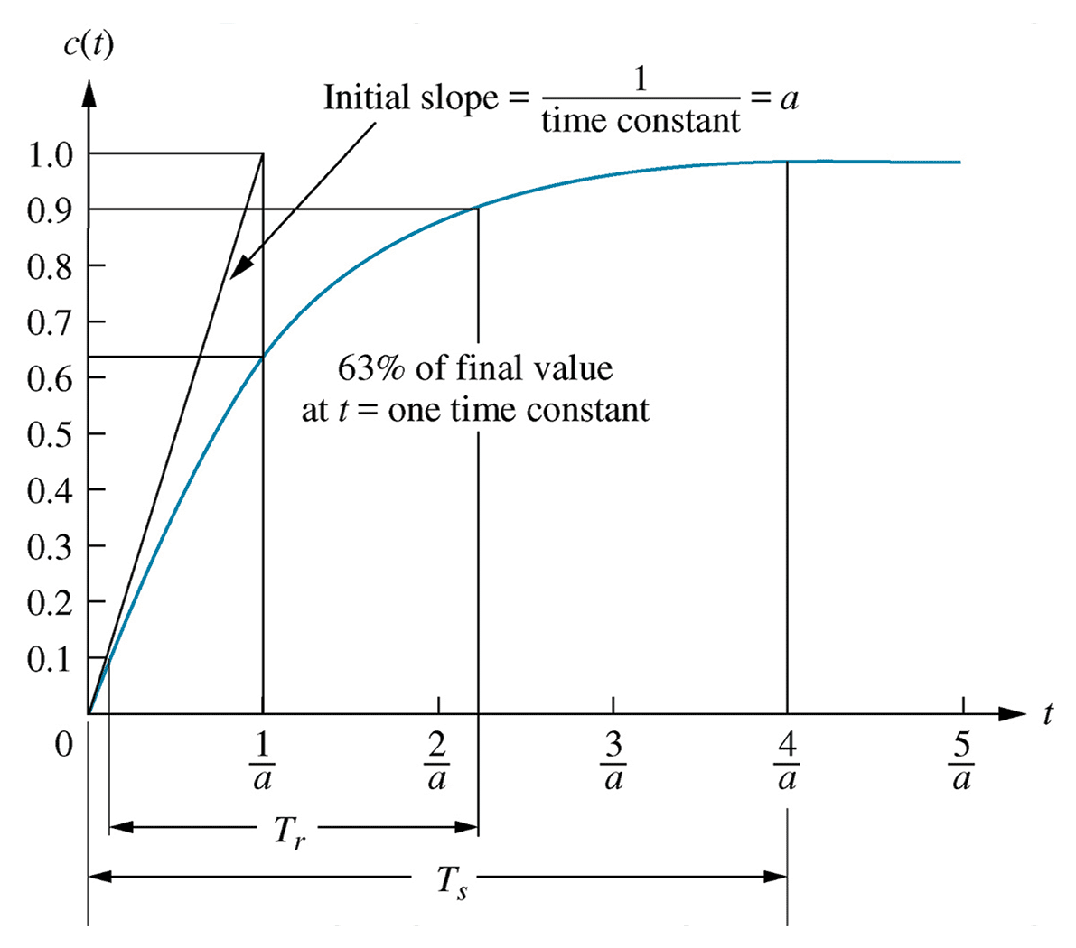
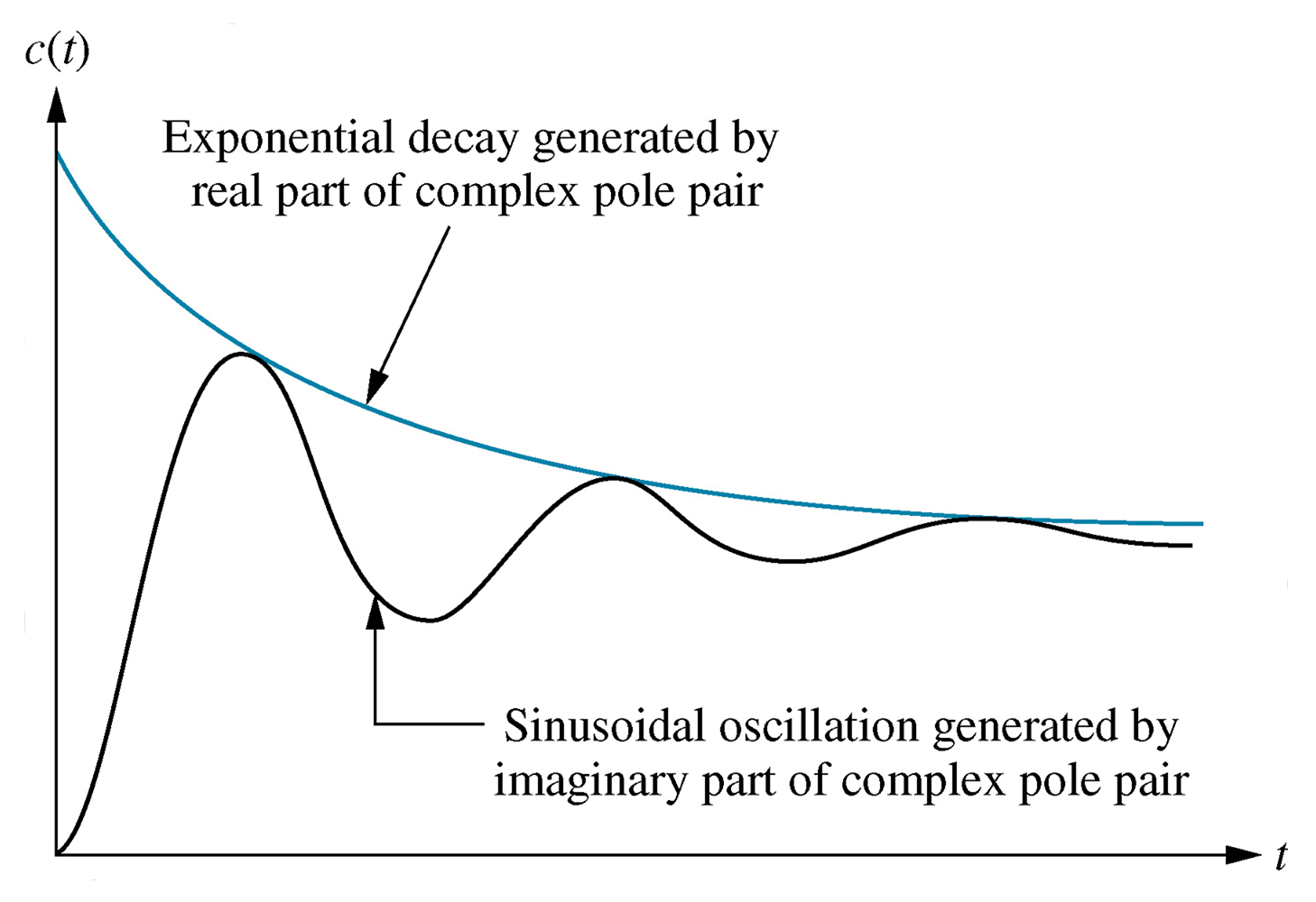
Pole location
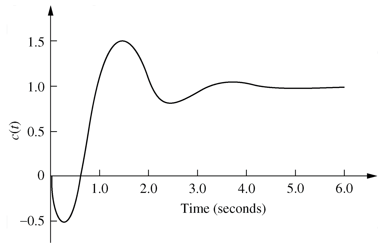
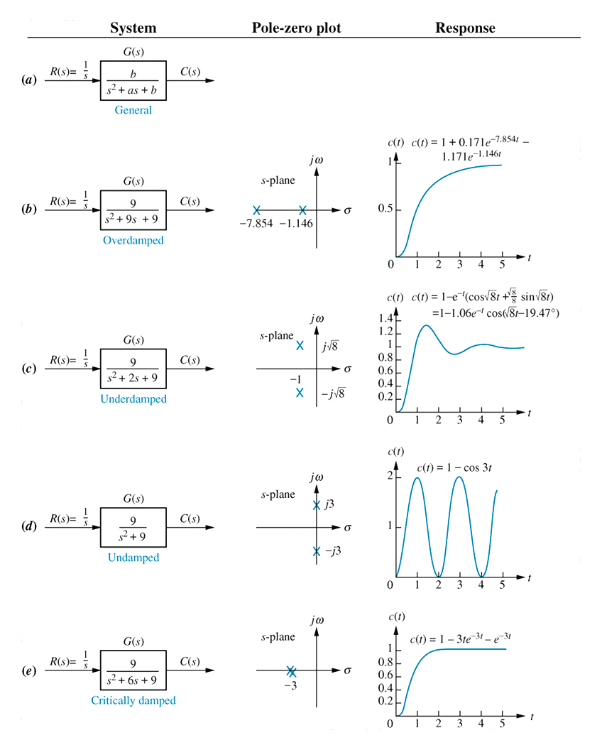
Every high order ODE, of order n, can be decomposed into a series of $n$ first order ODEs, as represented in a state space model.A high order ODE can be represented as a polynomial in $s$.Every high order polynomial can be represented as the product of first and second order terms with real coefficients.
Thus all systems can be considered as combinations of first and second order subsystems.
- Decomposition
-
38
- MATLAB
Generation of a pole-zero map and step response using MATLAB $^{123}$ for a system with unity negative feedback and open loop transfer function $G(s)$.
$G(s) = \large \frac{4(s+1)}{s(s+2)(s+3)}$
G = zpk(-1,[0,-2,-3],4)
Gc = feedback(G, 1)
figure(1); pzmap(Gc)
figure(2); step(Gc)
MATLAB1
MATLAB2
MATLAB3 - MATLAB
-
40
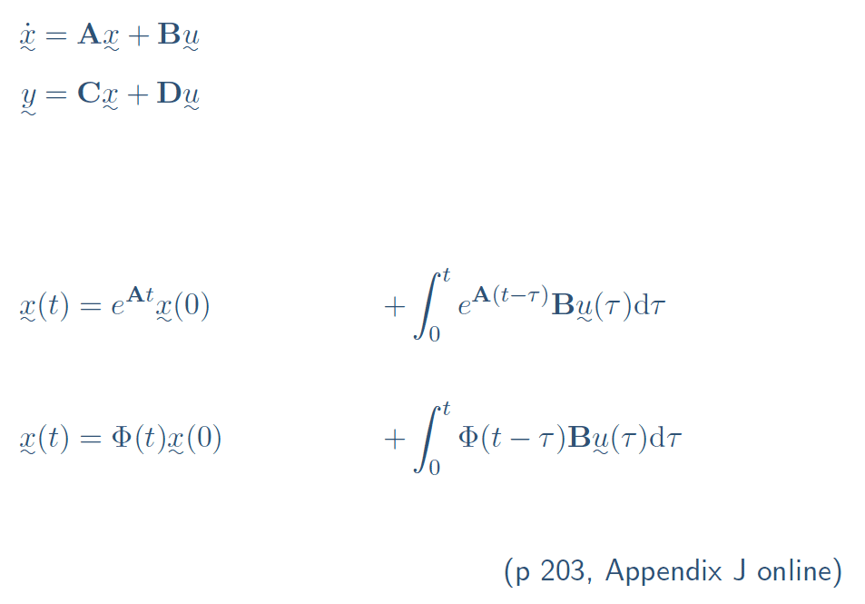
- State transition matrix
\begin{align*} \underset{\sim}{x}(t) &= e^{\mathrm{A}t}\underset{\sim}{x}(0) &+& \int_0^t e^{\mathrm{A}(t-\tau)}\mathrm{B}\underset{\sim}{u}(\tau) {\mathrm d}\tau \\ &&&\\ \underset{\sim}{x}(t) &= \Phi(t)\underset{\sim}{x}(0) &+& \int_0^t \Phi(t-\tau)\mathrm{B}\underset{\sim}{u}(\tau) {\mathrm d}\tau \\ \end{align*} $$\Phi(t)$$ is the state transition matrix and describes how states evolve in response to inputs (forced dynamics) and their current state (free, or natural, dynamics).
Free dynamics: \begin{align*} \mathcal{L}\left[\mathrm{x}(t)\right] &= \mathcal{L}\left[\Phi(t)\mathrm{x}(0)\right] &= \left(s\mathrm{I}-\mathrm{A}\right)^{-1}\mathrm{x}(0) \end{align*}42- Find $\phi(t)$
\begin{align*} \phi(t) = \mathcal{L}^{-1}\left[\Phi(s)\right] \\ \;\; \Phi(s) = \left(s\mathrm{I}-\mathrm{A}\right)^{-1} \\ \\ s, \mathrm{I} \; \textrm{and} \; \mathrm{A} \textrm{ are known.} \end{align*} $$\textrm{Procedure:} \qquad\qquad\qquad\qquad \\ \textrm{1. Find } \Phi(s) = \left(s\mathrm{I}-\mathrm{A}\right)^{-1}\\ \textrm{2. Find } \phi(t) = \mathcal{L}^{-1}\left[\Phi(s)\right] $$
44- Find $\phi(t) = \mathcal{L}^{-1}[\Phi(s)]$
\begin{align*} \Phi(s) = (s\mathrm{I}-\mathrm{A})^{-1} &= \frac{\begin{pmatrix} s+3 & 1 \\ -2 & s \end{pmatrix}}{s^2 + 3 s + 2} \\ &= \frac{\begin{pmatrix} s+3 & 1 \\ -2 & s \end{pmatrix}}{(s + 1)(s + 2)} \\ &= \begin{pmatrix} \frac{s+3}{(s+1)(s+2)} & \frac{1}{(s+1)(s+2)} \\ \frac{-2}{(s+1)(s+2)} & \frac{s}{(s+1)(s+2)} \end{pmatrix}\\ \end{align*} We need to use partial fractions.
46- Partial fractions
\begin{align*} \frac{s+3}{(s+1)(s+2)} &= \frac{ 2}{s+1} - \frac{1}{s+2} \\ \frac{ 1}{(s+1)(s+2)} &= \frac{ 1}{s+1} - \frac{1}{s+2} \\ \frac{ -2}{(s+1)(s+2)} &= \frac{-2}{s+1} + \frac{2}{s+2} \\ \frac{s }{(s+1)(s+2)} &= \frac{-1}{s+1} + \frac{2}{s+2} \end{align*}
48- Outputs: $t$-domain
\begin{align*} \phi(t) &= \begin{pmatrix} 2\,e^{-t}- e^{-2\,t} & e^{-t}- e^{-2\,t} \\ -2\,e^{-t}+2\,e^{-2\,t} & -e^{-t}+2\,e^{-2\,t} \end{pmatrix} \\ \end{align*}
\begin{align*} \underset{\sim}{y}(t) &= \mathrm{A} \underset{\sim}{x}(t) + \mathrm{B} \underset{\sim}{u}(t) \\ \underset{\sim}{x}(t) &= \phi(t)\underset{\sim}{x}(0) + \int_0^t \phi(t-\tau)\mathrm{B}\underset{\sim}{u}(\tau) \mathrm{d}\tau \end{align*}
Chapter 4 Summary
- Listen to the summary in the voiceover.
41- Example problem
Given the following state space model \begin{align*} \mathrm{A} &= \begin{pmatrix} 0 & 1 \\ -2 & -3 \end{pmatrix} & \mathrm{B} &= \begin{pmatrix} 0 \\ 0.5 \end{pmatrix} & \underset{\sim}{x}(0) &= \begin{pmatrix} 0 \\ 0 \end{pmatrix} \\ \mathrm{C} &= \begin{pmatrix} 1 & 0 \\ 0 & 1 \end{pmatrix} & \mathrm{D} &= \begin{pmatrix} 0 \\ 0 \end{pmatrix} &&\\ \end{align*}
1. Find the state transition matrix $\Phi(s)$ and $\phi(t)$
2. Sketch the response of output $y_1$ to a unit step input43- Find $\Phi(s) = \left(s\mathrm{I}-\mathrm{A}\right)^{-1}$
\begin{align*} \mathrm{A} &= \begin{pmatrix} 0 & 1 \\ -2 & -3 \end{pmatrix} \\ s \mathrm{I} - \mathrm{A} &= s\begin{pmatrix}1&0\\0&1\end{pmatrix}-\begin{pmatrix}0&1\\-2&-3\end{pmatrix} \\ &= \begin{pmatrix}s&0\\0&s\end{pmatrix}-\begin{pmatrix}0&1\\-2&-3\end{pmatrix} \\ &= \begin{pmatrix} s & -1 \\ 2 & s+3 \end{pmatrix} \\ \left(s \mathrm{I} - \mathrm{A}\right)^{-1} &= \frac{Adj(s \mathrm{I} - \mathrm{A})}{|s \mathrm{I} - \mathrm{A}|} \\ Adj(s\mathrm{I}-\mathrm{A}) = C^T &= \begin{pmatrix} s+3 & -2 \\ 1 & s \end{pmatrix}^T = \begin{pmatrix} s+3 & 1 \\ -2 & s \end{pmatrix} \\ |s\mathrm{I}-\mathrm{A}| &= (s)(s+3) - (-1)(2) = s^2 + 3 s + 2 \\ \end{align*}45- Partial fractions
\begin{align*} \frac{a s + b}{(s+1)(s+2)} &= \frac{A}{s+1} + \frac{B}{s+2} \end{align*}
\begin{align*} a s + b &= A(s+2) + B(s+1) \\ &= (A+B) s + (2A+B) \\ & \\ A+B &= a \\ 2A+B & = b \\ &\\ A &= b-a \\ B &= b- 2A = b-2(b-a) = 2a-b \end{align*}
47- $\Phi(s)$ as partial fractions
\begin{align*} \Phi(s) &= \begin{pmatrix} \frac{s+3}{(s+1)(s+2)} & \frac{1}{(s+1)(s+2)} \\ &\\ \frac{ -2}{(s+1)(s+2)} & \frac{s}{(s+1)(s+2)} \end{pmatrix} \\ &\\ &= \begin{pmatrix} \frac{ 2}{s+1}-\frac{1}{s+2} & \frac{ 1}{s+1}-\frac{1}{s+2} \\ &\\ \frac{-2}{s+1}+\frac{2}{s+2} & \frac{-1}{s+1}+\frac{2}{s+2)} \end{pmatrix} \end{align*} The outputs can be solved in the $t$ or $s$ domain.
49- Outputs: $s$-domain
\begin{align*} \underset{\sim}{Y}(s) &= \left(\mathrm{C} \mathrm{\phi}(s) \mathrm{B} + \mathrm{D}\right) \underset{\sim}{U}(s) \\ &\\ &= \left( \begin{pmatrix} 1 & 0 \\ 0 & 1 \end{pmatrix} \begin{pmatrix} \frac{s+3}{(s+1)(s+2)} & \frac{1}{(s+1)(s+2)} \\ \frac{ -2}{(s+1)(s+2)} & \frac{s}{(s+1)(s+2)} \end{pmatrix} \begin{pmatrix} 0 \\ 0.5 \end{pmatrix} + \begin{pmatrix} 0 \\ 0 \end{pmatrix} \right) \left( \frac{1}{s} \right) \\ &= \begin{pmatrix} \frac{1}{(s+1)(s+2)} \\ \frac{s}{(s+1)(s+2)} \end{pmatrix} \times \frac{0.5}{s} &\\ &= \begin{pmatrix} \frac{1}{4} \left(\frac{1}{s}-\frac{2}{s+1}+\frac{1}{s+2}\right) \\ \frac{1}{2} \left(\frac{1}{s+1}-\frac{1}{s+2}\right) \end{pmatrix} &\\ y_1(t) &= 0.25 - 0.5\,e^{-t} + 0.25\,e^{-2\,t} \\ y_2(t) &= 0.5\,e^{-t}-0.5\,e^{-2\,t} \end{align*}
- State transition matrix