Block Two
-

Chapter 5. Reduction of multiple subsystems
- block diagrams
- signal flow graphs
- similarity transforms *
Block diagrams and signal flow graphs
When developing or describing a control system, diagrams showing signal connections are of great benefit.
 Example 5.2, fig 5.11, p 243 / 241
\begin{align*} \frac{C(s)}{R(s)} &= \frac{G_1(s) G_3(s) [1+G_2(s)]} {[1+G_2(s)H_2(s)+G_1(s)G_2(s)H_1(s)][1+G_3(s)H_3(s)]} \end{align*}(Control Engineering 3 notes: weeks 1-6)
-
8
- Cascade state space
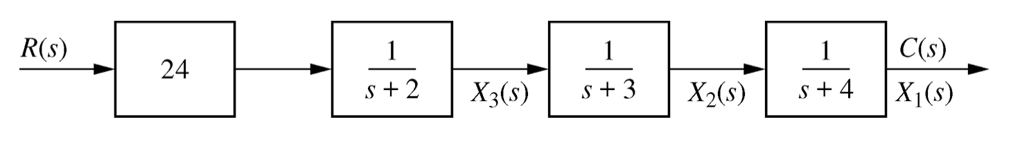
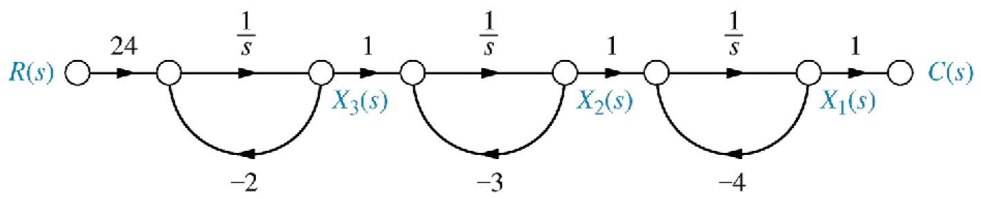 Fig 5.24(b), p258\begin{align*} \dot x_1 &= -4 x_1 && + x_2 && && \\ \dot x_2 &= && -3 x_2 && + x_3 && \\ \dot x_3 &= && && -2 x_3 && + 24 r \end{align*}
\begin{align*} \underset{\sim}{\dot x} &= \begin{pmatrix} -4 & 1 & 0 \\ 0 & -3 & 1 \\ 0 & 0 & -2 \end{pmatrix} \underset{\sim}{x} + \begin{pmatrix} 0 \\ 0 \\ 24 \end{pmatrix} r \\ \underset{\sim}{y} &= \begin{pmatrix} 1 & 0 & 0 \end{pmatrix} \underset{\sim}{ x} \end{align*}10- Controller canonical form
Controller canonical form: renumber phase variables in reverse order (p261).
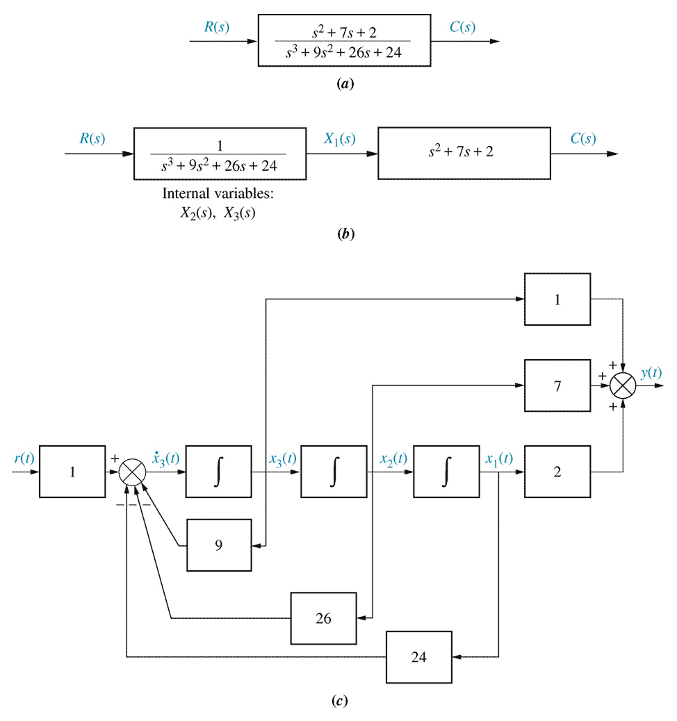
Phase variable form: \begin{align*} \underset{\sim}{\dot x} &= \begin{pmatrix} 0 & 1 & 0 \\ 0 & 0 & 1 \\ -24 & -26 & -9 \end{pmatrix} \underset{\sim}{x} + \begin{pmatrix} 0 \\ 0 \\ 1 \end{pmatrix} r \\ \underset{\sim}{y} &= \begin{pmatrix} 2 & 7 & 1 \end{pmatrix} \underset{\sim}{x} \end{align*} Controller canonical form: \begin{align*} \underset{\sim}{\dot x} &= \begin{pmatrix} -9 & -26 & -24 \\ 1 & 0 & 0 \\ 0 & 1 & 0 \end{pmatrix} \underset{\sim}{x} + \begin{pmatrix} 1 \\ 0 \\ 0 \end{pmatrix} r \\ \underset{\sim}{y} &= \begin{pmatrix} 1 & 7 & 2 \end{pmatrix} \underset{\sim}{x} \end{align*}1Chapter 5 - The Laplace transform
- Transfer functions
Decomposing block diagrams into regions with a single input and single output (possibly moving blocks to achieve this), block diagrams can be reduced to transfer functions for analysis in the frequency domain.
Block diagrams can also be used to develop Simulink models directly, using a series of “Transfer Function” blocks.
Signal flow diagrams are alternatives to block diagrams that emphasise the model variables (states, outputs, etc.) instead of the component transfer functions.3
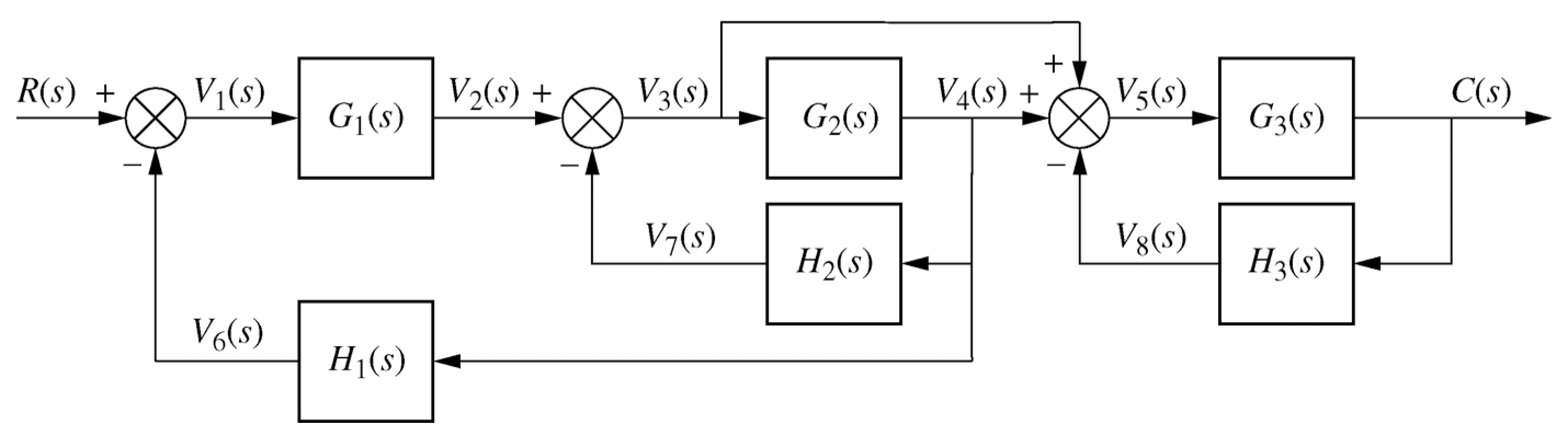
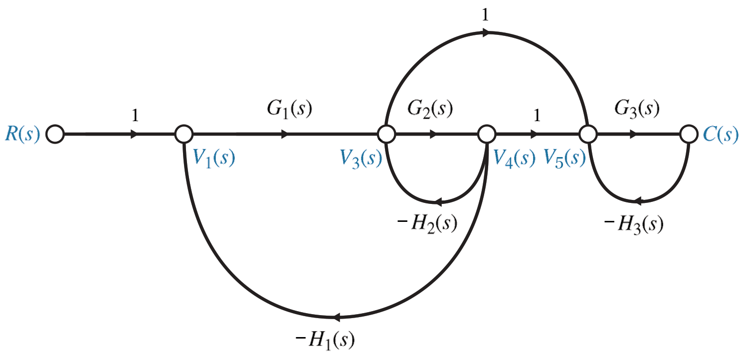
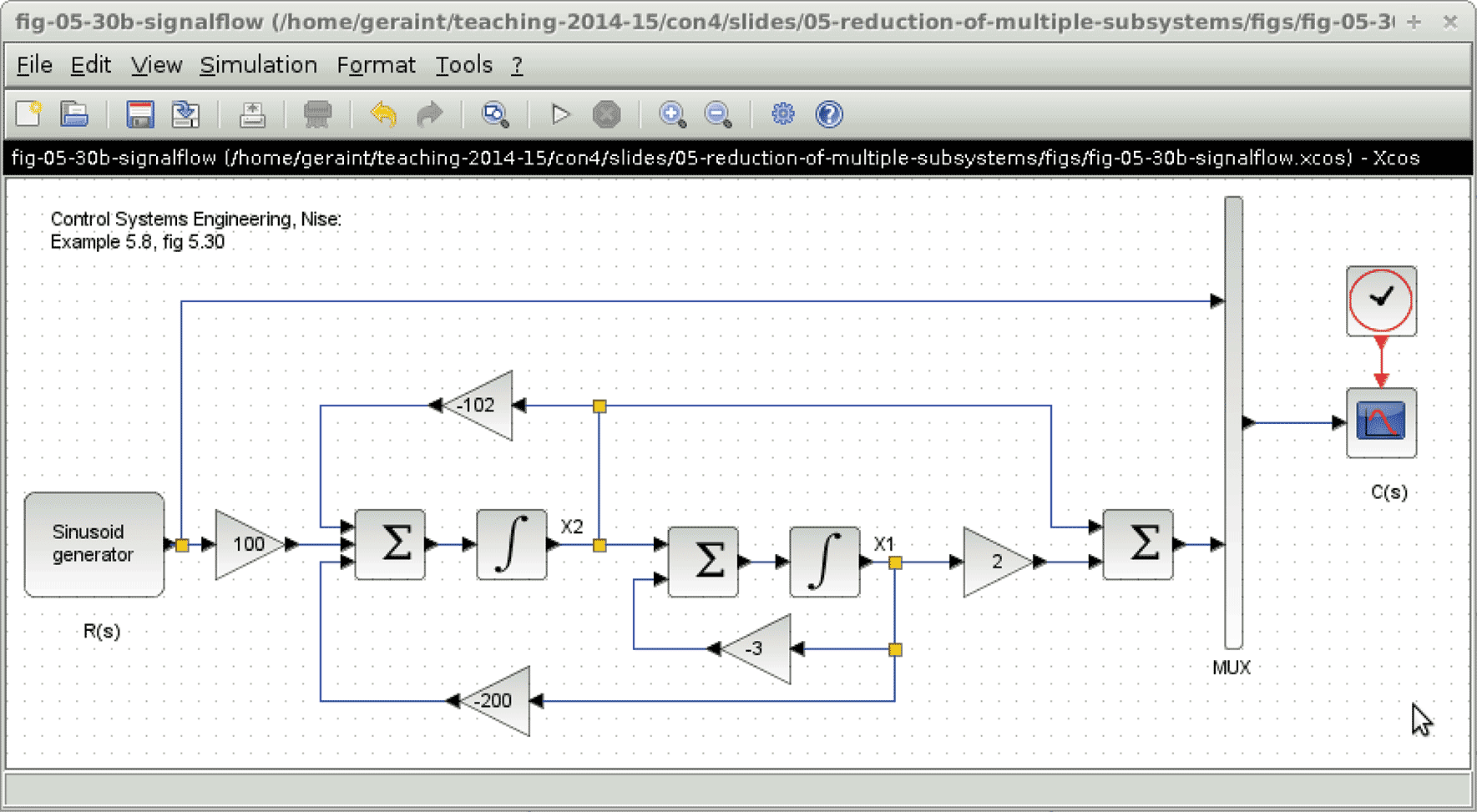
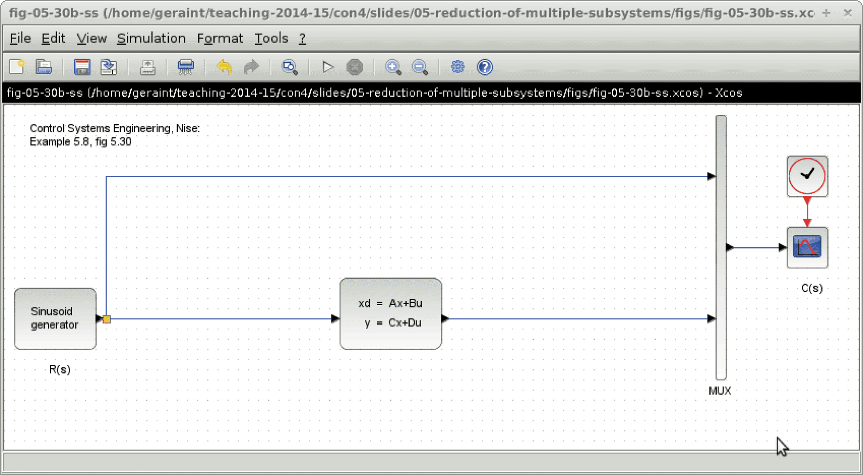
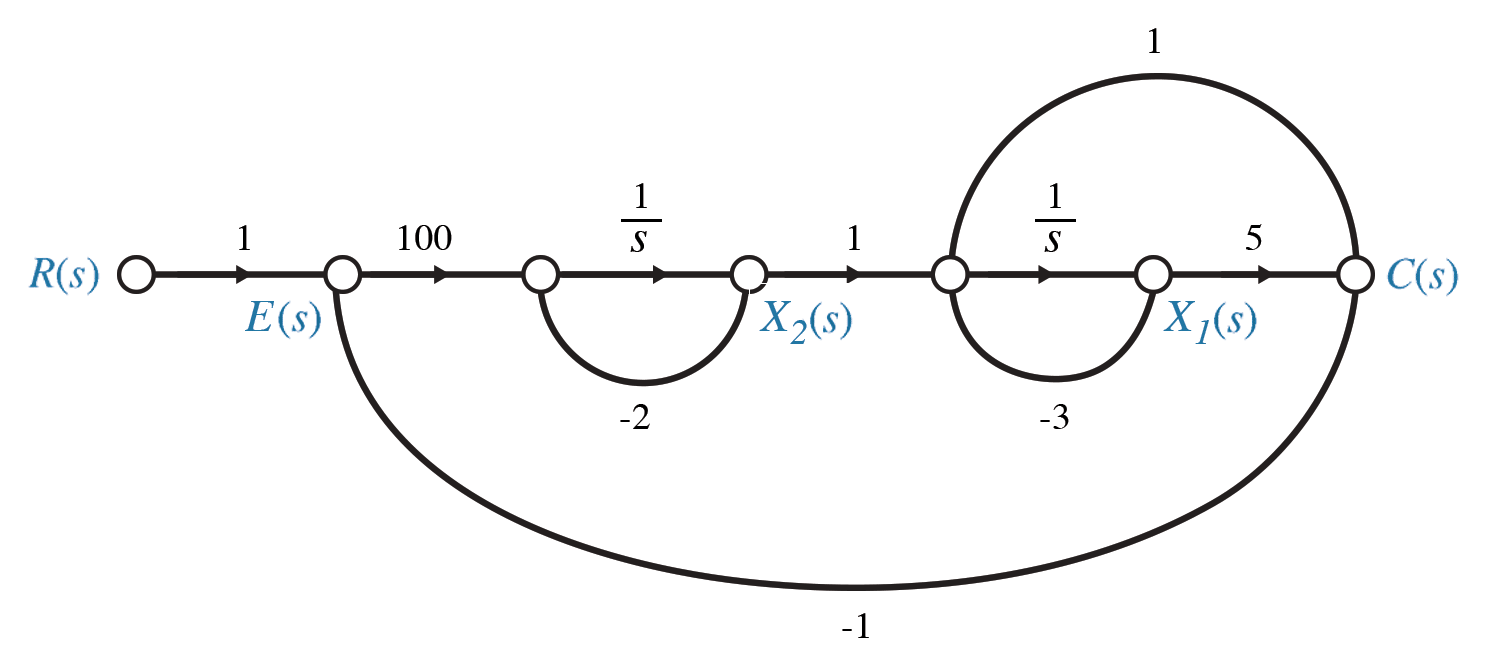 Example 5.8, fig 5.30, p 264 / 261
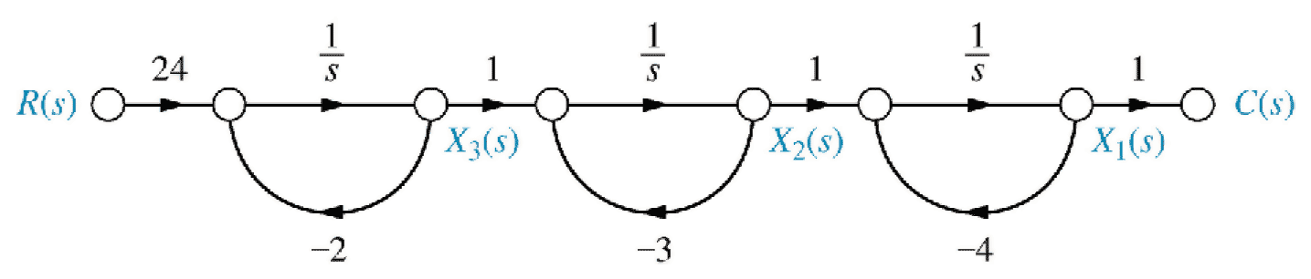
When drawing or analysing signal flow graphs, it is usually easiest to work right to left.
Start with the outputs and work backwards, adding states as necessary, an integrator ($1/s$) for each state, and the links between the states and their rates. \begin{align*} C &= 5 X_1 + \dot X_1 \qquad= 5 X_1 + (X_2 -3 X_1) \qquad= 2 X_1 + X_2 \\ \dot X_1 &= -3 X_1 + X_2 \\ \dot X_2 &= -2 X_2 + 100 (R - C) \qquad= -200 X_1 - 102 X_2 + 100 R \end{align*}5Alternative state space representations
- Phase variables
Phase variables are the states that we encountered in Chapter 3, where the states comprise successive derivatives of each other. \begin{align*} \ddot x_1 & &+ a &\dot x_1 & + b &x_1 & &=& c u \\ \downarrow& & &\downarrow& &\downarrow& && \\ \downarrow& & & \chi_2 & & \chi_1 & && \\ \downarrow& & &\downarrow& &\downarrow& && \\ \dot \chi_2& & & \dot \chi_1& & \chi_1 & && \end{align*} \begin{align*} \begin{pmatrix} \dot\chi_1 \\ \dot\chi_2 \end{pmatrix} &= \begin{pmatrix} 0 & 1 \\ -b& -a& \end{pmatrix} \begin{pmatrix} \chi_1 \\ \chi_2 \end{pmatrix} + \begin{pmatrix} 0 \\ c \end{pmatrix} u \end{align*}9- Parallel (decoupled) states
\begin{align*} \frac{C(s)}{R(s)} &= \frac{24}{(s+2)(s+3)(s+4)} = \frac{12}{s+2}-\frac{24}{s+3}+\frac{12}{s+4} \end{align*} \begin{align*} \underset{\sim}{\dot x} &= \begin{pmatrix} -2 & 0 & 0 \\ 0 & -3 & 0 \\ 0 & 0 & -4 \end{pmatrix} \underset{\sim}{x} + \begin{pmatrix} 12 \\ -24 \\ 12 \end{pmatrix} r \\ \underset{\sim}{y} &= \begin{pmatrix} 1 & 1 & 1 \end{pmatrix} \underset{\sim}{x} \end{align*}
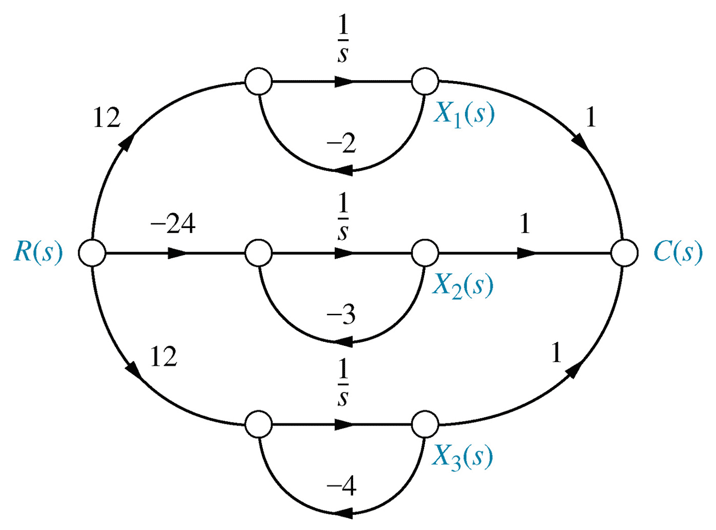 Fig 5.25, p25911
- Observer canonical form
Observer canonical form: transpose of controller canonical form (p263).
Controller canonical: \begin{align*} \underset{\sim}{\dot x} &= \begin{pmatrix} -9 & -26 & -24 \\ 1 & 0 & 0 \\ 0 & 1 & 0 \end{pmatrix} \underset{\sim}{x} + \begin{pmatrix} 1 \\ 0 \\ 0 \end{pmatrix} r \\ \underset{\sim}{y} &= \begin{pmatrix} 1 & 7 & 2 \end{pmatrix} \underset{\sim}{x} \end{align*} Observer canonical: \begin{align*} \underset{\sim}{\dot x} &= \begin{pmatrix} -9 & 1 & 0 \\ -26 & 0 & 1 \\ -24 & 0 & 0 \end{pmatrix} \underset{\sim}{x} + \begin{pmatrix} 1 \\ 7 \\ 2 \end{pmatrix} r \\ \underset{\sim}{y} &= \begin{pmatrix} 1 & 0 & 0 \end{pmatrix} \underset{\sim}{x} \end{align*} - Cascade state space
-
13
- Uncoupling systems
Matrix diagonalisation can be used to diagonalise the state matrix.
A diagonalised state matrix implies a decoupled system, in which each state is affected only by itself and the inputs; not the other states.
Decoupled systems are generally easier to analyse and develop control systems for.15- Diagonalised matrix
If matrix $\mathrm{P}$ comprises the eigenvectors of matrix $\mathrm{A}$, then the matrix product $\mathrm{P^{-1}}\mathrm{A}\mathrm{P}$ will be a diagonal matrix.
Hence this transformation can be used to decouple a state space model.17- Diagonalisation with Matlab
A = [ 0, 1; -2, -3]
B = [ 0; 1 ]
C = [ 1, 0 ]
D = [ 0 ]
[ P, Ad ] = eig(A)
assert((inv(P)*A*P - Ad) = zeros(size(A))
Bd = inv(P)*B
Cd = C*P
G1 = ss( A, B, C, D)
figure(1)
step(G1)
G2 = ss( Ad, Bd, Cd, D)
figure(2)
step(G2)
12Similarity transforms
- Similarity transforms
``Oh, what a tangled web we weave. When first we desire to'' ... model engineering systems.
(apologies to Walter Scott)
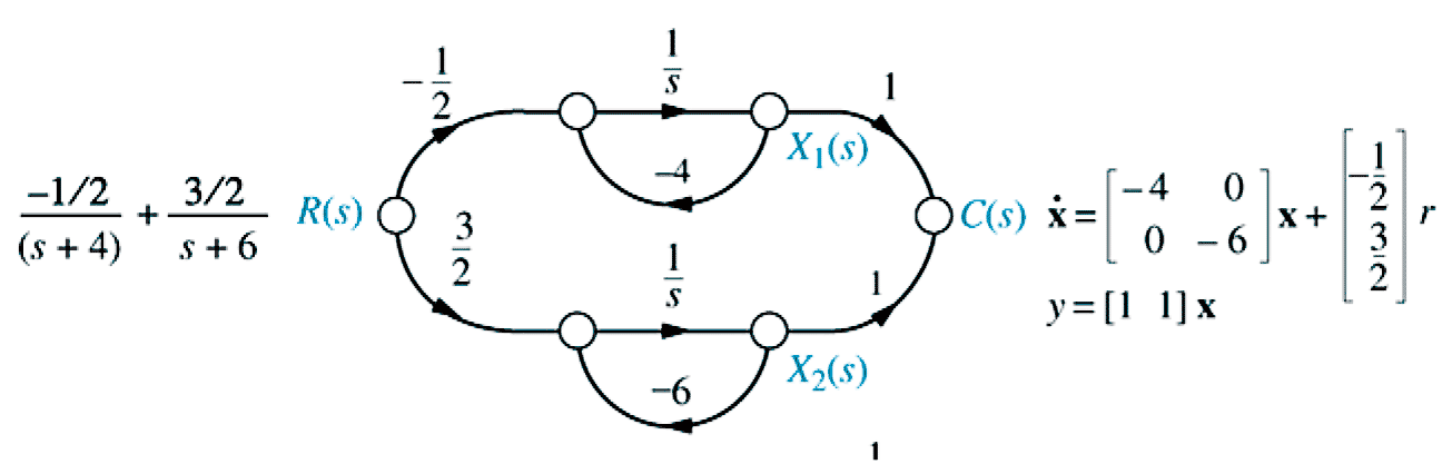 Fig 5.31, p265
\begin{align*} \underset{\sim}{\dot x} &= \begin{pmatrix} -4 & 0 \\ 0 & -6 \end{pmatrix} \underset{\sim}{x} + \begin{pmatrix} -\frac{1}{2} \\ \frac{3}{2} \end{pmatrix} \underset{\sim}{r} & \underset{\sim}{y} &= \begin{pmatrix} 1 & 1 \end{pmatrix} \underset{\sim}{x} \end{align*}14- Similarity Transformation ($\S$5.8, p266)
Coupled state space system: \begin{align*} \underset{\sim}{\dot x} &= \mathrm{A} \underset{\sim}{x} + \mathrm{B} \underset{\sim}{u} \\ \underset{\sim}{y} &= \mathrm{C} \underset{\sim}{x} + \mathrm{D} \underset{\sim}{u} \end{align*}
Let $\underset{\sim}{z} = \mathrm{P^{-1}} \underset{\sim}{x} \;$ (i.e. $\underset{\sim}{x} \rightarrow \mathrm{P}\underset{\sim}{z}$, $\underset{\sim}{\dot x} \rightarrow \mathrm{P}\underset{\sim}{ \dot z}$).
\begin{align*} \mathrm{P} \underset{\sim}{\dot z} &= \mathrm{A} \mathrm{P} \underset{\sim}{z} + \mathrm{B} \underset{\sim}{u} \\ \underset{\sim}{y} &= \mathrm{C} \mathrm{P} \underset{\sim}{z} + \mathrm{D} \underset{\sim}{u} \end{align*}
\begin{align*} \underset{\sim}{\dot z} &= \mathrm{P^{-1}} \mathrm{A} \mathrm{P} \underset{\sim}{z} + \mathrm{P^{-1}} \mathrm{B} \underset{\sim}{u} \\ \underset{\sim}{y} &= \mathrm{C} \mathrm{P} \underset{\sim}{z} + \mathrm{D} \underset{\sim}{u} \end{align*}16- Diagonalisation example
State space model:
\begin{align*} \mathrm{A}&=\begin{pmatrix}0&1\\-2&-3\end{pmatrix}& \mathrm{B}&=\begin{pmatrix}0\\1\end{pmatrix}\\ \mathrm{C}&=\begin{pmatrix}1&0\end{pmatrix}& \mathrm{D}&=\begin{pmatrix}0\end{pmatrix} \end{align*} $eig \; (\mathrm{A}): |\lambda I - A|=0$ \begin{align*} \left|\begin{matrix} \lambda & -1 \\ 2 & \lambda+3 \end{matrix}\right| & = 0 & \lambda^2 + 3\lambda + 2 &= 0 \\ &&(\lambda + 1)(\lambda +2) &= 0 \end{align*}
\begin{align*} \left|\begin{matrix} \lambda & -1 \\ 2 & \lambda+3 \end{matrix}\right| & = 0 & \lambda = -1 \; \text{or} \; -2 \end{align*}
\begin{align*} \begin{pmatrix} -1 & -1 \\ 2 & -1+3 \end{pmatrix} \begin{pmatrix}x_1\\x_2\end{pmatrix} &= \begin{pmatrix}0\\0\end{pmatrix} \; \implies \underset{\sim}{x} &= \begin{pmatrix} -1 \\ 1 \end{pmatrix} \\ \begin{pmatrix} -2 & -1 \\ 2 & -2+3 \end{pmatrix} \begin{pmatrix}x_1\\x_2\end{pmatrix} &= \begin{pmatrix}0\\0\end{pmatrix} \; \implies \underset{\sim}{x} &= \begin{pmatrix} -1 \\ 2 \end{pmatrix} \\ \mathrm{P} &= \begin{pmatrix} -1 & -1 \\ 1 & 2 \end{pmatrix} \\ \mathrm{P}^{-1}\mathrm{A}\mathrm{P} &= \begin{pmatrix} -1 & 0 \\ 0 & -2 \end{pmatrix} \end{align*} - Uncoupling systems
-
19
Routh Hurwitz criteria
- Design tool
The Matlab command pzmap can show the pole locations of a given system, to allow stability and transient performance analysis, but is less helpful when controller parameters are unknown.
The Routh-Hurwitz stability criteria allow constraints on unknown parameters to be calculated, hence assisting in the design process.
These constraint equations can be used to guide the design of physical system parameters or controller gains.21- Routh array construction
The Routh array has as many rows as the order of the characteristic polynomial, i.e. the highest power of $s$.
The coefficients of $s$ (in descending order) are placed alternately in the first two rows of the array.
Elements in subsequent rows are calculated using the two rows above, making use of the left-most column and the column to the right.
Routh array (2nd order)
\begin{align*} G(s) &= \frac{\mathrm{blah}}{s^2+a_1 s+a_0} \end{align*} \begin{array}{l|ll} s^2: & 1 & a_0 \\ s^1: & a_1 & 0 \\ s^0: & b_1 \end{array} \begin{align*} b_1 &= -\frac{\left| \begin{matrix} 1 & a_0 \\ a_1 & 0 \end{matrix} \right|} {a_1} \end{align*}
Routh array (3nd order)
\begin{align*} G(s) &= \frac{\mathrm{blah}}{s^3+a_2 s^2+a_1 s+a_0} \end{align*} \begin{array}{l|ll} s^3: & 1 & a_1 \\ s^2: & a_2 & a_0 \\ s^1: & b_1 & 0 \\ s^0: & c_1 \end{array} \begin{align*} b_1 &= -\frac{\left| \begin{matrix} 1 & a_1 \\ a_2 & a_0 \end{matrix} \right|} {a_2} & c_1 &= -\frac{\left| \begin{matrix} a_2 & a_0 \\ b_1 & 0 \end{matrix} \right|} {b_1} \end{align*}
Routh array (4nd order)
\begin{align*} G(s) &= \frac{\mathrm{blah}}{s^4+a_3 s^3+a_2 s^2+a_1 s+a_0} \end{align*} \begin{array}{l|lll} s^4: & 1 & a_2 & a_0\\ s^3: & a_3 & a_1 & 0\\ s^2: & b_1 & b_2 & 0\\ s^1: & c_1 & 0 \\ s^0: & d_1 & 0 \end{array} \begin{align*} b_1 &= -\frac{\left| \begin{matrix} 1 & a_2 \\ a_3 & a_1 \end{matrix} \right|} {a_3} & b_2 &= -\frac{\left| \begin{matrix} 1 & a_0 \\ a_3 & 0 \end{matrix} \right|} {a_3} \\ c_1 &= -\frac{\left| \begin{matrix} a_3 & a_1 \\ b_1 & b_2 \end{matrix} \right|} {b_1} & d_1 &= -\frac{\left| \begin{matrix} b_1 & b_2 \\ c_1 & 0 \end{matrix} \right|} {c_1} \end{align*}23State space stability
- State space stability
Recall the state transition matrix: \begin{align*} \phi(s) &= (s\mathrm{I}-\mathrm{A})^{-1} \\ &= \frac{Adj(s\mathrm{I}-\mathrm{A})}{|s\mathrm{I}-\mathrm{A}|} \end{align*} The system poles are located at the eigenvalues of matrix $\mathrm{A}$.
For stability we require that the eigenvalues of the state matrix $\mathrm{A}$ should be located in the left half plane (LHP) of the $s$-domain, i.e. negative real part.
Unlike mathematicians, as Engineers you should be able to take systems with complex eigenvalues and eigenvectors in your stride. You have been studying such systems for years without realising it!18
Chapter 6. Stability
- Routh Hurwitz criteria
- Stability in state space
20- Routh-Hurwitz criteria
For stability, three criteria must be satisfied. These criteria are based on the denominator of the closed loop transfer function, i.e. the characteristic polynomial.
1. All coefficients of $s$ must be non-zero
2. No sign changes in the coefficients of $s$
3. No sign changes in the first column of the Routh array
Criterion 1 arises because systems with missing coefficients of $s$ imply poles on the imaginary ($j\omega$) axis, implying marginal stability. For design purposes, we can consider marginally stable systems to be unstable.
Criterion 2 arises because the number of sign changes equals the number of poles in the right half plane (RHP); we require none!22- Special cases
Zeros in the first column of the Routh array would lead to division by zero. These should be replaced by $\large \epsilon$, representing a very small number.
Rows of zeros imply that the CLTF has an even polynomial as a factor. These can be dealt with by generating an even polynomial from the row above and differentiating, as shown in Example 6.8, p316.
These special cases will not appear in the exam.
- Design tool
-
25
Steady state errors
- Context
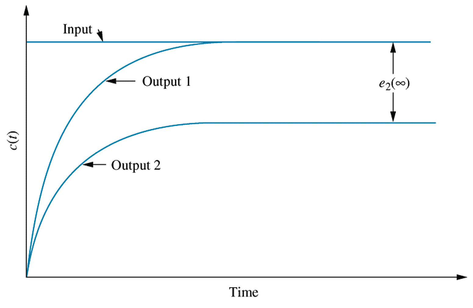
Along with analysis of stability and transient performance, steady state error often forms an integral part of the specification for a system's behaviour.
Evaluation of steady state error only makes sense in the context of a stable system. Analysing steady state error in an unstable system would lead to perverse results.
In the $s$-domain, steady state errors can be analysed using the Final Value Theorem.
It can be instructive to consider the steady state errors arising from systems subjected to various standard inputs, such as step, ramp and parabolic inputs.29- Steady state error for unit step input
\begin{align*} e_{step}(\infty) &= \lim_{s\rightarrow 0} \frac{s R(s)}{1+G(s)} & R(s) &= \frac{1}{s} \\ \ \\ e_{step}(\infty) &= \lim_{s\rightarrow 0} \frac{\require{cancel}\cancel{s} \times 1 / \cancel{s}}{1+G(s)} \\ &= \frac{1}{1+\lim_{s \rightarrow 0} G(s)} \end{align*}
The term $\lim_{s\rightarrow 0}G(s)$ is known as the DC gain of the forward path in electrical engineering, or its steady state gain more generally.31- Integral action
If the open loop transfer function $G(s)$ has one or more uncancelled poles at the origin (i.e. a pure integrator), there will be no steady state error in response to a step input.
Proof: \begin{align*} \text{Let } G(s) &= \frac{(s+z_1)(s+z_2)\ldots}{s^n(s+p_1)(s+p_2)\ldots}\\ \ \\ \lim_{s\rightarrow 0} G(s) &= \frac{(z_1)(z_2)\ldots}{0^n(p_1)(p_2)\ldots} \rightarrow \infty \\ \ \\ e_{step}(\infty) &= \frac{1}{1+\lim_{s\rightarrow 0}G(s)} \rightarrow \frac{1}{1+\infty} \rightarrow 0 \end{align*}33- Steady state error for parabola input
\begin{align*} e_{parabola}(\infty) &= \lim_{s\rightarrow 0} \frac{s R(s)}{1+G(s)} & R(s) &= \frac{1}{s^3} \\ e_{parabola}(\infty) &= \lim_{s\rightarrow 0} \frac{\cancel{s} \times 1 / s^{\cancelto{2}{3}}}{1+G(s)} \\ &= \lim_{s\rightarrow 0} \frac{1}{s^2+s^2 G(s)} \\ &= \frac{1}{\lim_{s \rightarrow 0} s^2 G(s)} \end{align*} To eliminate steady state error for a parabolic input, there must be three or more uncancelled poles at the origin of the open loop (forward path) transfer function.24
Chapter 7 - Steady state errors
- Steady state error specifications
- Steady state errors for systems in state space
28- Final value theorem
Recall the Final value theorem: \begin{align*} f(\infty) &= \lim_{s\rightarrow 0} s F(s) \\ \end{align*}
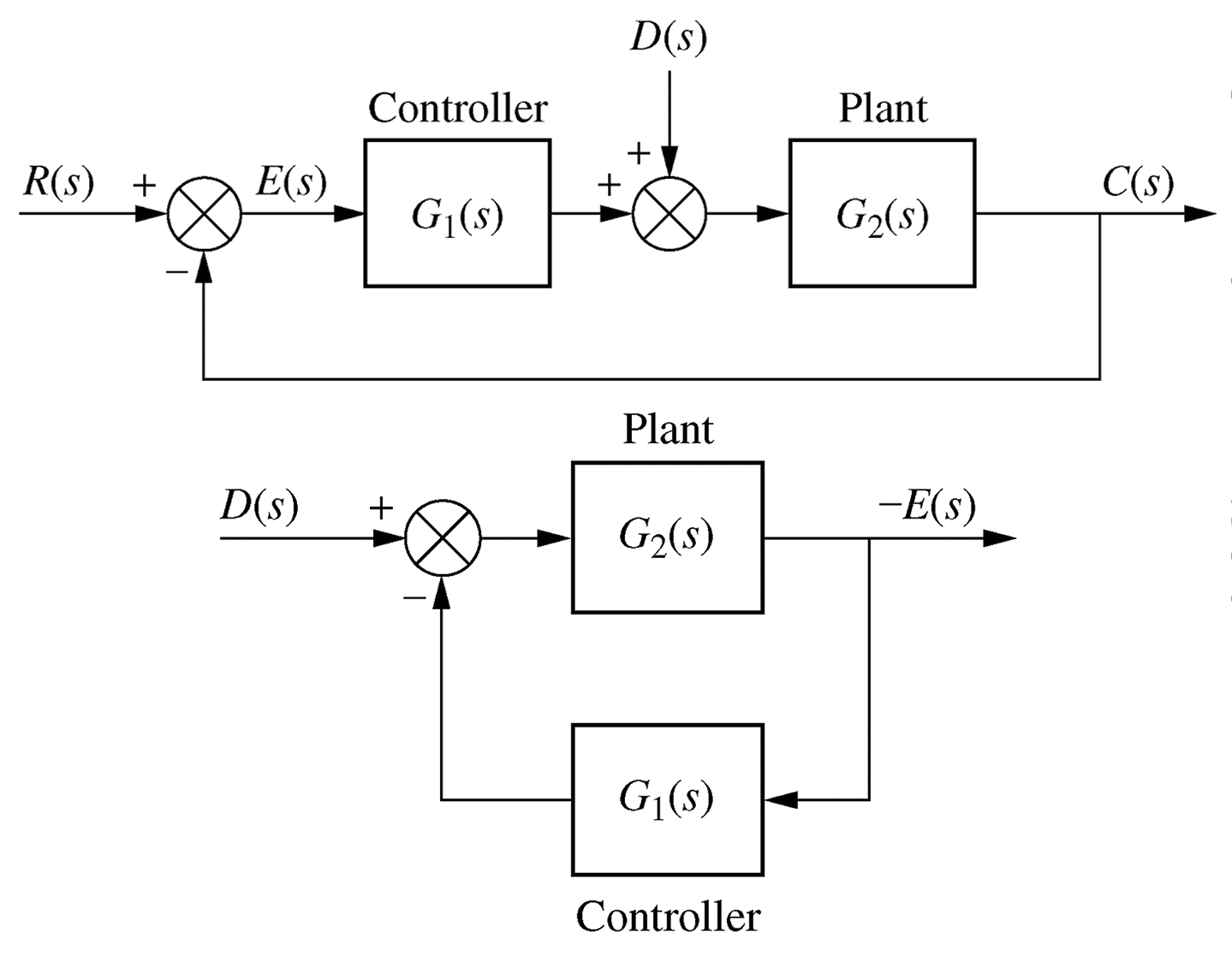
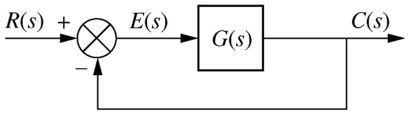 Fig 7.3b, p342 / 336: open loop TF G(s) with unity feedback
\begin{align*} E(s) &= \frac{R(s)}{1+G(s)} & e(\infty) &= \lim_{s\rightarrow 0} \frac{s R(s)}{1+G(s)} \end{align*}30- Using $T(s)$ instead
Note, if we calculate the closed loop transfer function $T$ (or $G_c(s)$) instead, we can derive a similar result: \begin{align*} T(s) &= \frac{G(s)}{1+G(s)} \\ \\ y_{step}(\infty) &= \lim_{s\rightarrow 0} s T(s) R(s) \\ \\ e_{step}(\infty) &= \lim_{s\rightarrow 0} \cancel{s} \left(1 - T(s) \right) \cancel{R(s)} & R(s) &= \frac{1}{s} \\ \\ e_{step}(\infty) &= 1 - \lim_{s\rightarrow 0} T(s) \end{align*}32- Steady state error for unit ramp input
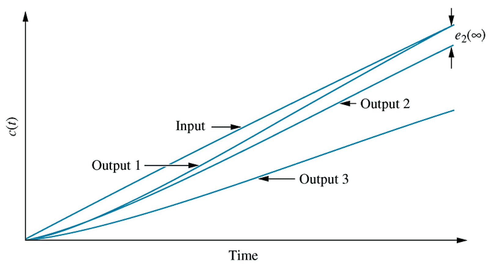
\begin{align*} e_{ramp}(\infty) &= \lim_{s\rightarrow 0} \frac{s R(s)}{1+G(s)} & R(s) &= \frac{1}{s^2} \\ e_{ramp}(\infty) &= \lim_{s\rightarrow 0} \frac{\cancel{s} \times 1 / s^{\cancel{2}}}{1+G(s)} \\ &= \lim_{s\rightarrow 0} \frac{1}{s+s G(s)} \\ &= \frac{1}{\lim_{s \rightarrow 0} s G(s)} \end{align*}
To eliminate steady state error for a ramp input, there must be two or more uncancelled poles at the origin of the open loop (forward path) transfer function.
- Context
-
37
- Sensitivity
Sensitivity analysis allows determination of the dependence of a function on a change of parameter.
Sensitivity $S_{F:P}$ gives the change in value of function $F$ due to a change in parameter $P$ and is defined: \begin{align*} S_{F:P} &= \lim_{\Delta P\rightarrow 0} \frac{\text{Fractional change in} F}{\text{Fractional change in} P} \\ \ \\ &= \lim_{\Delta P\rightarrow 0} \frac{P\Delta F}{F\Delta P} \\ \ \\ &= \frac{P}{F} \frac{\delta F}{\delta P} \end{align*}39Steady state error in state space
- Final value theorem in state space
\begin{align*} e(\infty) &= \lim_{s\rightarrow 0} s E(s) \\ \ \\ E(s) &= R(s) - C(s) = \left(1 - (\mathrm{C}\mathrm{\Phi}(s)\mathrm{B}+\mathrm{D})\right) R(s) \\ \mathrm{\Phi}(s) &= (s\mathrm{I}-\mathrm{A})^{-1} \\ \ \\ e(\infty) &= \lim_{s\rightarrow 0} s (1-\mathrm{C}\mathrm{\Phi}(s)\mathrm{B}-\mathrm{D}) R(s) \end{align*}34- Static error constants
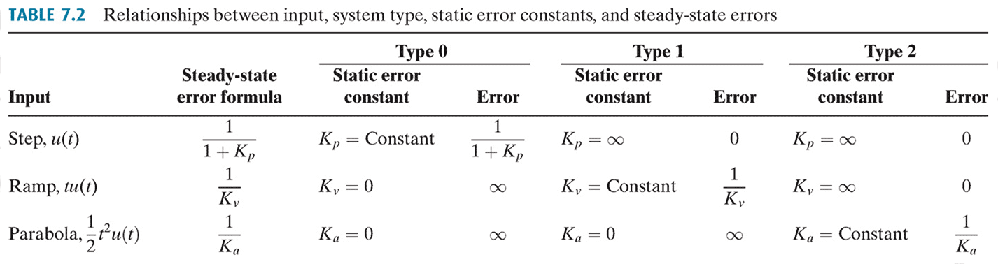
The three limit terms obtained in the steady state error calculations for the step, ramp and parabolic input are known collectively as static error constants.
\begin{align*} K_p &= \lim_{s\rightarrow 0} G(s) & \quad \text{Position constant} \\ \ \\ K_v &= \lim_{s\rightarrow 0} s G(s) & \quad \text{Velocity constant} \\ \ \\ K_a &= \lim_{s\rightarrow 0} s^2 G(s) & \quad \text{Acceleration constant} \\ \end{align*}38- Sensitivity example 7.10 (1/3)
\begin{align*} T(s) &= \frac{K}{s^2+a s+K} & S_{T:a} &= \frac{a}{T} \frac{\delta T}{\delta a} \\ \end{align*}
Given a system with uncertain parameter $a$, determine the sensitivity of the closed loop transfer function $T(s)$ to a change in $a$
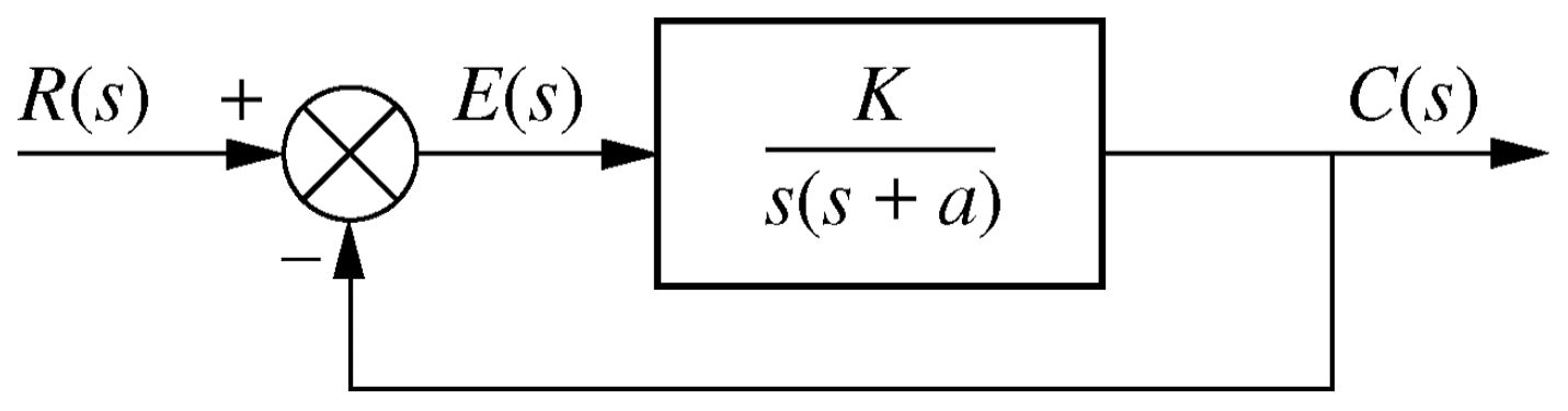 Fig 7.19, p362 / 355: Example 7.10
● Sensitivity example 7.10 (2/3)
\begin{align*} T(s) &= \frac{K}{s^2+a s+K} & S_{T:a} &= \frac{a}{T} \frac{\delta T}{\delta a} \\ \end{align*}
\begin{align*} \frac{\delta T}{\delta a} &= \frac{\delta}{\delta a} \left(K(s^2+a s+K)^{-1}\right) \\ &= (-1)\times K(s^2+a s +K)^{(-1-1)}\times \frac{\delta}{\delta a}\left(s^2+a s+K)\right)\\ &= \frac{- K}{(s^2+a s+K)^2} \times s \\ &= \frac{- K s}{(s^2+a s + K)^2} \end{align*}
● Sensitivity example 7.10 (3/3)
\begin{align*} T(s) &= \frac{K}{s^2+a s+K} & S_{T:a} &= \frac{a}{T} \frac{\delta T}{\delta a} \\ \end{align*}
\begin{align*} S_{T:a} &= \frac{a}{T} \times \frac{-K s}{(s^2+a s + K)^2} \\ &= \frac{a}{\frac{\require{cancel}\cancel{K}}{\cancel{s^2+as+K}}} \times \frac{-\cancel{K} s}{(s^2+a s + K)^{\cancel{2}}} \\ &= \frac{-as}{s^2+as+K} \end{align*} Note that increasing $K$ decreases the sensitivity of
$T(s)$ to $a$.40- Steady state error for a unit step input
For a unit step $R(s) = 1/s$
\begin{align*} e_{step}(\infty) &= \lim_{s\rightarrow 0} (1-\mathrm{C}\mathrm{\Phi}(s)\mathrm{B}-\mathrm{D}) \end{align*} Quick and dirty (works for a step input!): \begin{align*} \lim_{s\rightarrow 0} \mathrm{\Phi}(s) &= \lim_{s\rightarrow 0}(\cancelto{0}{s}\mathrm{I}-\mathrm{A})^{-1} \\ &= (-\mathrm{A})^{-1} \\ \ \\ e_{step}(\infty) &= 1+\mathrm{C}\mathrm{A}^{-1}\mathrm{B}-\mathrm{D} \end{align*} - Sensitivity