Block Three
-

Chapter 12 - Design via state space
- Controller design
- Controllability
- Observability
-
2
- Plant representation
A system with an $n^\text{th}$ order characteristic equation requires $n$ adjustable controller parameters: \begin{align*} s^n + a_{n-1} s^{n-1} + \ldots + a_1 s + a_0 &= 0 \end{align*} Henceforth, let us assume that the transmission matrix $\mathrm{D}$ is zero, and omit it from the state space representation. Let us also assume a single input $u$ and output $y$: \begin{align*} \underset{\sim}{\dot x} &= \mathrm{A}\underset{\sim}{x} + \mathrm{B} u & y &= \mathrm{C}\underset{\sim}{x} \end{align*}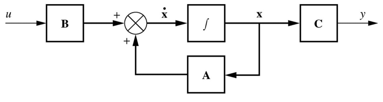 6
6- Matrix dimensions
\begin{align*} \underset{\sim}{\dot x} &= (\mathrm{A}-\mathrm{B}\mathrm{K})\underset{\sim}{x} + \mathrm{B} r & y &= \mathrm{C}\underset{\sim}{x} \end{align*} Matrix $\mathrm{K}$ must have as many columns as there are rows in $\underset{\sim}{x}$
i.e. the number of states.
Matrix $\mathrm{K}$ must have as many rows as there are columns in $\mathrm{B}$
i.e. the number of inputs.
For a SISO system, \begin{align*} \mathrm{K} &= \begin{pmatrix} k_1 & k_2 & \cdots & k_n \end{pmatrix} \end{align*} The dimensions can be easily adapted for MIMO systems.8- Pole placement with Matlab
The Matlab command place() can calculate the matrix $\mathrm{K}$.
$\tt {K = place(A,B,p)}$
where $\tt{A}$ and $\tt{B}$ are the state and input matrices of the plant and $\tt{p}$ is an array of pole locations.
uk.mathworks.com/help/10Example
- Pole placement example
A plant is defined as a state space system of equations: \begin{align*} \underset{\sim}{\dot x} &= \begin{pmatrix} -1 & 0 \\ 0 & -2 \end{pmatrix} \underset{\sim}{x} + \begin{pmatrix} 1 \\ 1 \end{pmatrix} u & y &= \begin{pmatrix} 1 & 1 \end{pmatrix} \underset{\sim}{x} \end{align*}
Design a full state feedback controller such that the closed loop system has damping ratio $\zeta=0.8$ and natural frequency $\omega_n=1$ rad/s.12- Example: block diagram and equations
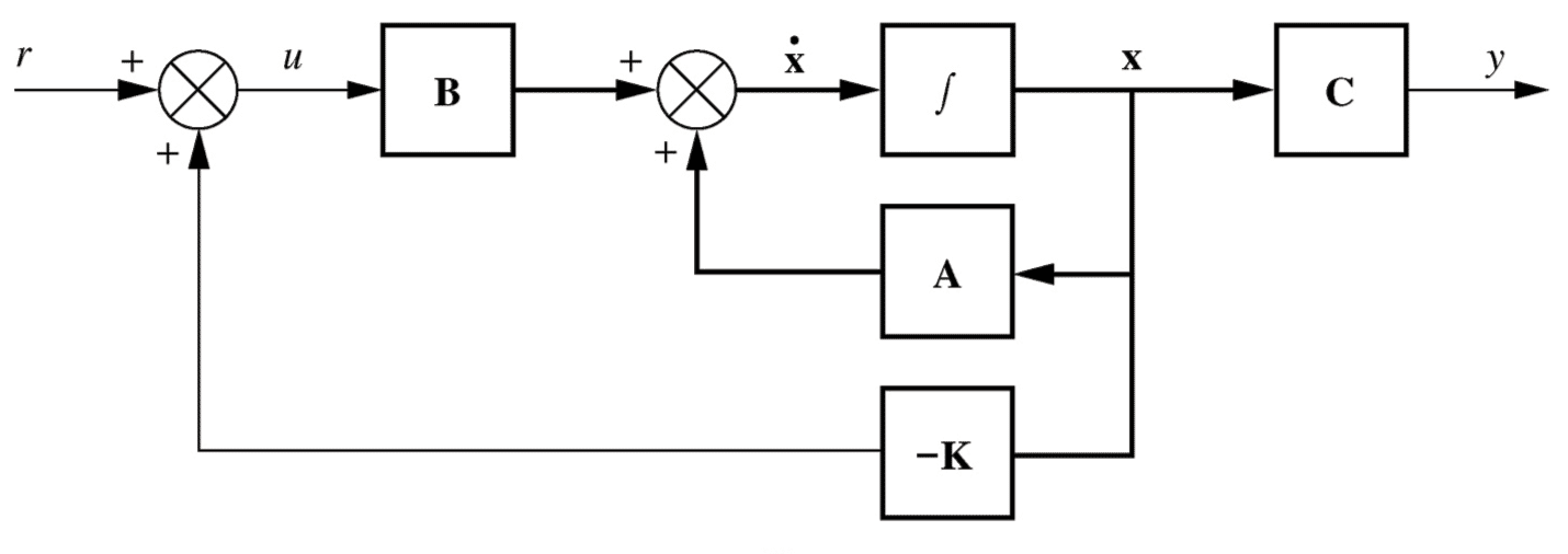
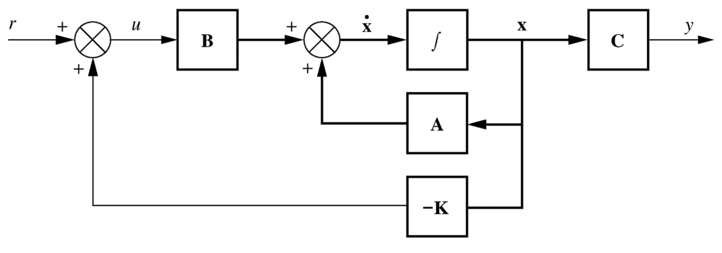
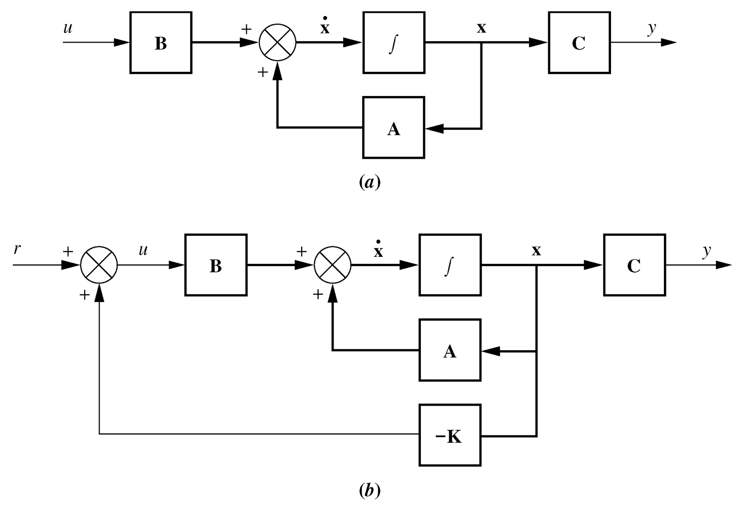
Plant: \begin{align*} \underset{\sim}{\dot x} &= \mathrm{A}\underset{\sim}{x} + \mathrm{B}u & y &= \mathrm{C}\underset{\sim}{x} \end{align*} Control law: \begin{align*} u &= r - \mathrm{K}\underset{\sim}{x} \end{align*} Controlled system: \begin{align*} \underset{\sim}{\dot x} &= (\mathrm{A}-\mathrm{B}\mathrm{K})\underset{\sim}{x} + \mathrm{B}r & y &= \mathrm{C}\underset{\sim}{x} \end{align*} Controlled system poles: \begin{align*} |s\mathrm{I} - (\mathrm{A}-\mathrm{B}\mathrm{K})| &= 0 \end{align*} Examples continue on the next tab >1- Pole placement
Controller design
the $s$-plane, to meet a desired specification.
Placement of $n$ poles requires a controller with $n$ parameters that can be adjusted.
Pole placement makes use of the state space representation. It is assumed that all system states can be measured (or otherwise known1)
1A Luenberger observer can be constructed using a similar method to pole placement.5- System equations
\begin{align*} \underset{\sim}{\dot x} &= \mathrm{A}\underset{\sim}{x} + \mathrm{B} u & y &= \mathrm{C}\underset{\sim}{x} \\ \\ u &= r - \mathrm{K}\underset{\sim}{x} \\ \\ \underset{\sim}{\dot x} &= \mathrm{A}\underset{\sim}{x} + \mathrm{B} (r-\mathrm{K}\underset{\sim}{x}) \\ \\ \underset{\sim}{\dot x} &= (\mathrm{A}-\mathrm{B}\mathrm{K})\underset{\sim}{x} + \mathrm{B} r & y &= \mathrm{C}\underset{\sim}{x} \end{align*}7- State transition matrix
The state transition matrix for the controlled system can be calculated in a similar manner to the uncontrolled plant.
Uncontrolled plant \begin{align*} \underset{\sim}{\dot x} &= \mathrm{A}\underset{\sim}{x} + \mathrm{B}\underset{\sim}{u} & y &= \mathrm{C}\underset{\sim}{x} \\ \Phi(s) &= (s\mathrm{I}-\mathrm{A})^{-1} \end{align*} Controlled system \begin{align*} \underset{\sim}{\dot x} &= (\mathrm{A}-\mathrm{B}\mathrm{K})\underset{\sim}{x} + \mathrm{B}\underset{\sim}{r} & y &= \mathrm{C}\underset{\sim}{x} \\ \Phi(s) &= \left(s\mathrm{I}-(\mathrm{A}-\mathrm{B}\mathrm{K})\right)^{-1} \end{align*} The controlled system poles are therefore located at \begin{align*} |s\mathrm{I}-(\mathrm{A}-\mathrm{B}\mathrm{K})| &= 0 \end{align*}9- The most difficult part ...
The mathematics of pole placement is relatively easy.
Determining where to place the poles is harder. This requires your engineering insight and understanding of the system requirements to develop an appropriate controller specification. Your knowledge of the $s$-plane should guide you.
Decisions about where to place the poles will have consequences for actuator requirements, and hence cost and/or efficiency implications.
As a rule of thumb, the further you try to move poles from their natural locations, the greater the power requirements.11- Example: procedure
1. Draw a block diagram of the controller structure
2. Derive the system equations (plant and control law)
3. Find the characteristic equation
4. Develop a target specification and its characteristic equation i.e. determine the target pole locations
5. Equate coefficients to map the controlled system to the target
6. Solve to find the controller gain matrix $\mathrm{K}$
7. Verify
- Plant representation
-
14
- Example: target characteristic equation
Controlled system characteristic equation: \begin{align*} s^2 + (k_1+k_2+3)s + 2+2k_1+k_2+ \require{cancel}\cancel{k_1k_2} -\cancel{k_1k_2} &= 0 \end{align*} Target specification: \begin{align*} \zeta& =0.8 & \omega_n &= 1\text{ rad/s} \end{align*} Target characteristic equation: \begin{align*} s^2 + 2\zeta\omega_n s + \omega_n^2 &= s^2 + 1.6 s + 1 = 0 \end{align*} Equating coefficients: \begin{align*} s^0&:& 1 &= 2+2k_1+k_2 \\ s^1&:& 1.6 &= k_1+k_2+3 \end{align*}
16- Example: verification
Target: \begin{align*} s^2 + 1.6 s + 1 &= 0 \end{align*} Controlled system: \begin{align*} s^2 + (k_1+k_2+3)s + 2+2k_1+k_2 &= 0 \end{align*} Substitute $k_1 = 0.4$ and $k_2 = -1.8$: \begin{align*} s^2 + (0.4-1.8+3)s + 2+2(0.4)+(-1.8) &= 0 \\ s^2 + 1.6 s + 1 &= 0 \end{align*} Thus the controlled system matches the target.20- Controllability matrix
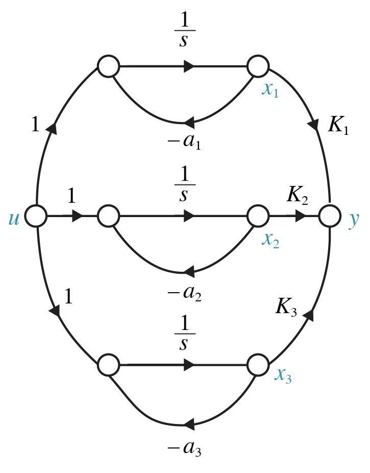
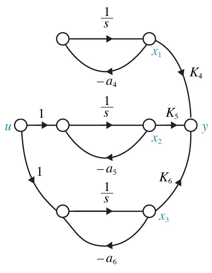
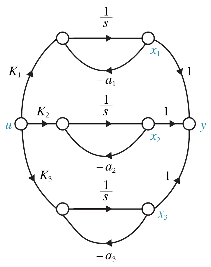
For a system in parallel form (i.e. decoupled), the controllability of each state can be readily determined by inspection of the signal graph or state and input matrices $\mathrm{A}$ and $\mathrm{B}$.
For a general state space system, its controllability can be determined by calculating the determinant of the controllability matrix. If the determinant is non-zero (i.e. the matrix is of full rank), the system is controllable. \begin{align*} \mathcal{C} &= \begin{pmatrix} \mathrm{B} & \mathrm{A}\mathrm{B} & \cdots & \mathrm{A}^{n-1}\mathrm{B} \end{pmatrix} \end{align*}13- Example: controlled system poles
Controlled system poles: \begin{align*} |s\mathrm{I} - (\mathrm{A}-\mathrm{B}\mathrm{K})| &= 0 \end{align*} The system has two states ($\mathrm{A}$ is size $2\times 2$), hence two controller gains: \begin{align*} \mathrm{K} &= \begin{pmatrix} k_1 & k_2 \end{pmatrix} \\ \mathrm{B}\mathrm{K} &= \begin{pmatrix} 1 \\ 1 \end{pmatrix} \begin{pmatrix} k_1 & k_2 \end{pmatrix} = \begin{pmatrix} k_1 & k_2 \\ k_1 & k_2 \end{pmatrix} \end{align*} \begin{align*} |s\mathrm{I} - (\mathrm{A}-\mathrm{B}\mathrm{K})| &= \left| s\begin{pmatrix} 1 & 0 \\ 0 & 1 \end{pmatrix} - \begin{pmatrix} -1 & 0 \\ 0 & -2 \end{pmatrix} + \begin{pmatrix} k_1 & k_2 \\ k_1 & k_2 \end{pmatrix} \right| = 0 \end{align*}
\begin{align*} |s\mathrm{I} - (\mathrm{A}-\mathrm{B}\mathrm{K})| &= \left| s\begin{pmatrix} 1 & 0 \\ 0 & 1 \end{pmatrix} - \begin{pmatrix} -1 & 0 \\ 0 & -2 \end{pmatrix} + \begin{pmatrix} k_1 & k_2 \\ k_1 & k_2 \end{pmatrix} \right| = 0 \end{align*} \begin{align*} \left| \begin{matrix} s+1+k_1 & k_2 \\ k_1 & s+2+k_2 \end{matrix} \right| &= 0 \end{align*} \begin{align*} (s+1+k_1)(s+2+k_2) - k_1 k_2 &= 0 \end{align*} \begin{align*} s^2 + (k_1+k_2+3)s + 2+2k_1+k_2+ \require{cancel} \cancel{k_1k_2} -\cancel{k_1k_2} &= 0 \end{align*}15- Example: solving for $\mathrm{K}$
\begin{align*} s^1&:& 1.6 &= k_1+k_2+3 &\implies& k_1+k_2 = -1.4\\ &&\implies& k_2 = -1.4-k_1 \\ s^0&:& 1 &= 2+2k_1+k_2 &\implies& 1 = 2k_1+(-1.4-k_1)+2 \\ &&\implies& k_1 = 0.4 \end{align*} Hence $k_1=0.4$, $k_2=-1.8$ and the desired control law is: \begin{align*} u &= r - \begin{pmatrix} 0.4 & -1.8 \end{pmatrix} \begin{pmatrix} x_1 \\ x_2 \end{pmatrix} \end{align*}17Controllability
- Controllability
In order to control the states, and hence outputs, of a system it is necessary that the system be controllable.
Controllability is a test of whether it is possible to manipulate each state independently using the available inputs. - Example: target characteristic equation
-
24
- Observability matrix
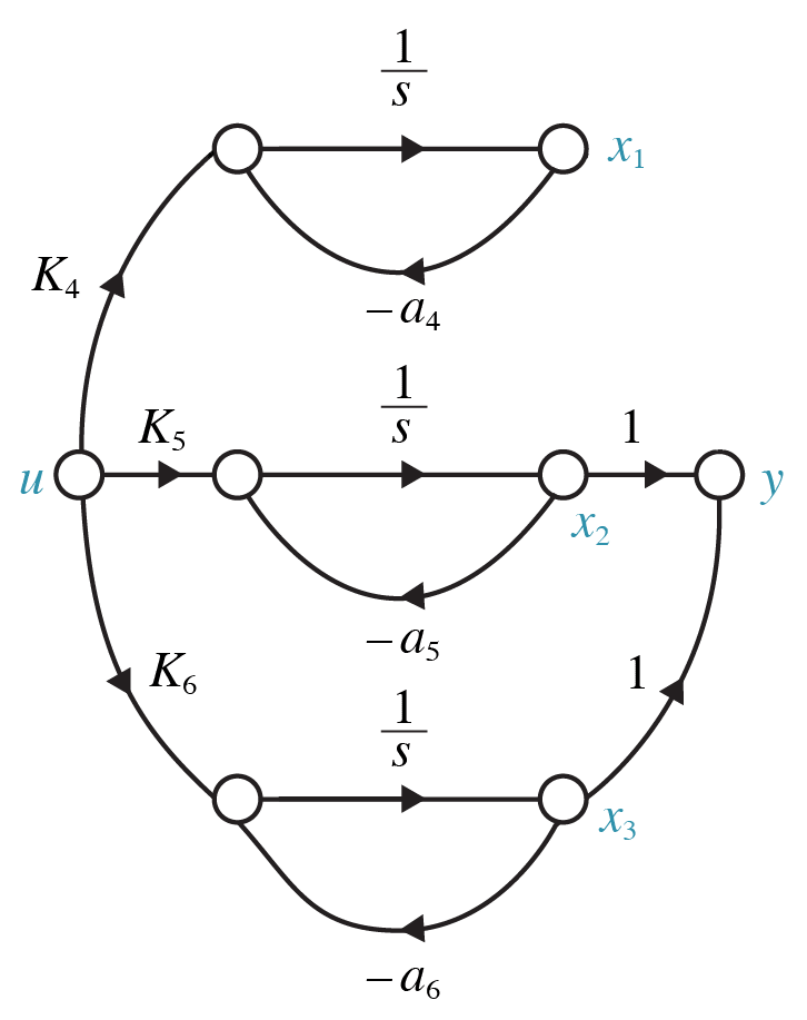
For a system in parallel form (i.e. decoupled), the observability of each state can be readily determined by inspection of the signal graph or state and output matrices $\mathrm{A}$ and $\mathrm{C}$.
For a general state space system, its observability can be determined by calculating the determinant of the observability matrix. If the determinant is non-zero (i.e. the matrix is of full rank), the system is observable. \begin{align*} \mathcal{O} &= \begin{pmatrix} \mathrm{C} \\ \mathrm{C}\mathrm{A} \\ \vdots \\ \mathrm{C}\mathrm{A}^{n-1} \end{pmatrix} \end{align*}26- Integral action with pole placement
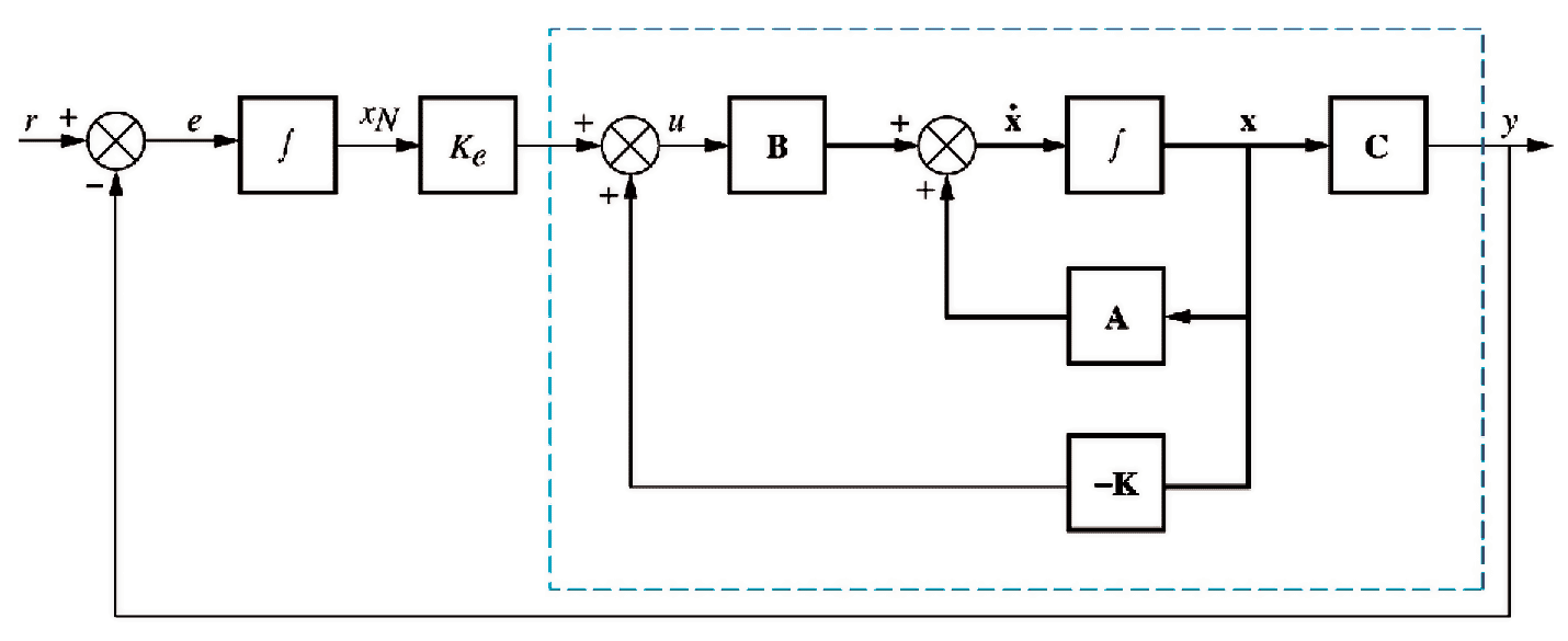 Figure 12.21, p700 / 684
\begin{align*} \begin{pmatrix}\underset{\sim}{\dot x}\\\dot x_n\end{pmatrix} &= \begin{pmatrix} \mathrm{A}-\mathrm{B}\mathrm{K} & \mathrm{B}k_e \\ -\mathrm{C} & 0 \end{pmatrix} \begin{pmatrix} \underset{\sim}{x} \\ x_n \end{pmatrix} + \begin{pmatrix} \mathrm{0} \\ 1 \end{pmatrix} r \\ y &= \begin{pmatrix} \mathrm{C} & 0 \end{pmatrix} \begin{pmatrix} \underset{\sim}{x} \\ x_N \end{pmatrix} \end{align*}28- Example: transfer function
\begin{align*} T(s) &= \mathrm{C} \mathrm{\Phi}(s) \mathrm{B} & \mathrm{\Phi}(s) &= \left(s\mathrm{I}-(\mathrm{A}-\mathrm{B}\mathrm{K})\right)^{-1} \end{align*} \begin{align*} \Phi(s) &= \frac{Adj \;\left(s\mathrm{I}-(\mathrm{A}-\mathrm{B}\mathrm{K})\right)}{|s\mathrm{I}-(\mathrm{A}-\mathrm{B}\mathrm{K})|} \end{align*} The determinant is known from previous analysis (the target characteristic equation): \begin{align*} |s\mathrm{I}-(\mathrm{A}-\mathrm{B}\mathrm{K})| &= s^2+2\zeta\omega_ns+\omega_n^2 = s^2+1.6s+1 \end{align*} The adjoint is the cofactor matrix transposed.30- Example: transfer function
\begin{align*} T(s) &= \frac{ \begin{pmatrix} 1 & 1 \end{pmatrix} \begin{pmatrix} s+2+k_2 & -k_2 \\ -k_1 & s+1+k_1 \end{pmatrix} \begin{pmatrix} 1 \\ 1 \end{pmatrix} }{s^2+1.6s+1} \\ \\ &= \frac{ \begin{pmatrix} 1 & 1 \end{pmatrix} \begin{pmatrix} s+2 \\ s+1 \end{pmatrix} }{s^2+1.6s+1} \\ \\ &= \frac{(s+2)+(s+1)}{s^2+1.6s+1} \\ \\ &= \frac{2s+3}{s^2+1.6s+1} \end{align*}
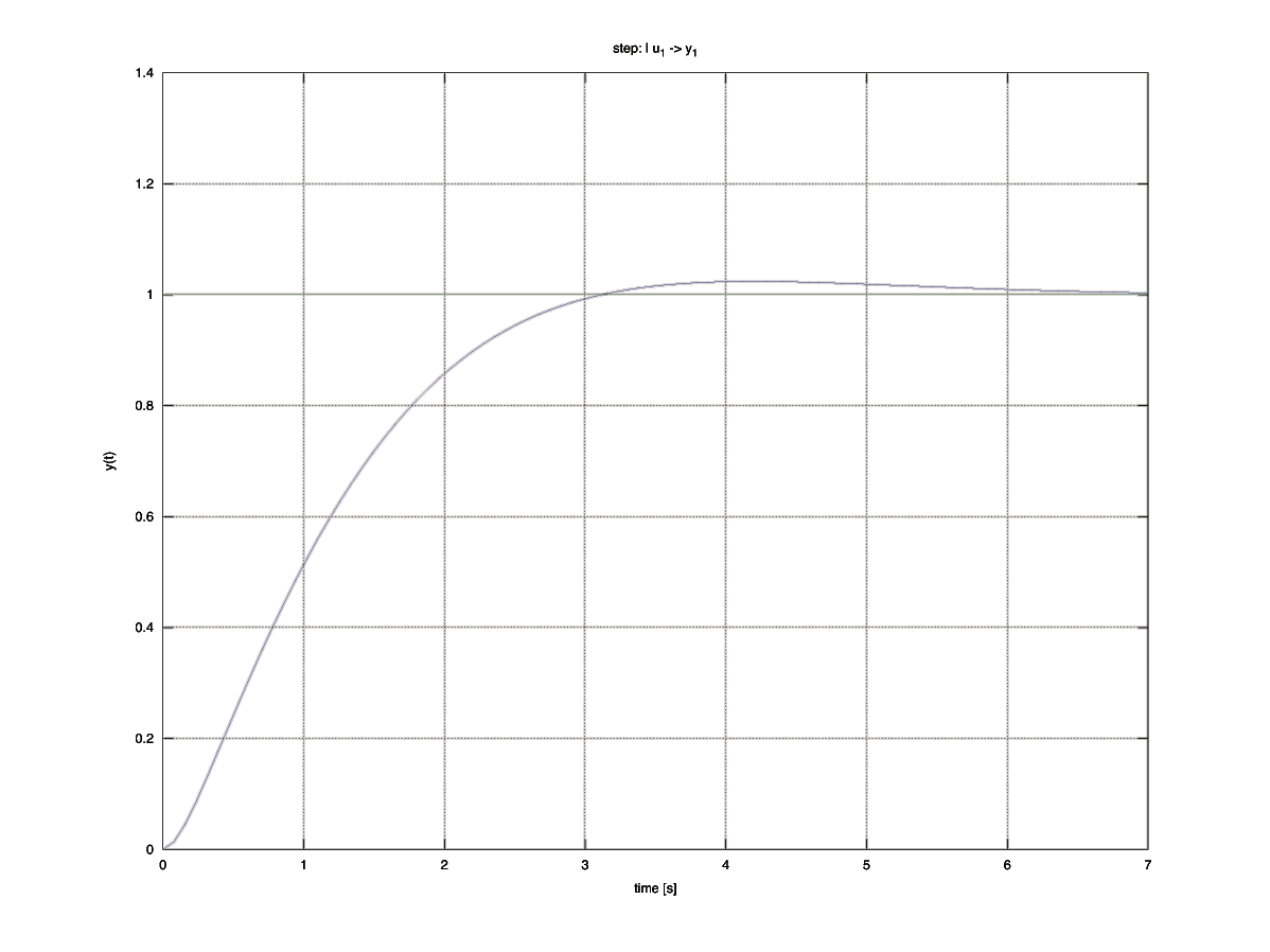
32- Example: result
The steady state error is non-zero in response to a step input. This suggests that the controller must be modified. The steady state error can be eliminated by introducing ``integral action'' into the forward path of the system, i.e. sufficient uncancelled poles at the origin based on the type of input.
For a step input, 1 uncancelled pole at the origin will suffice. For a ramp input, 2 are required. For a parabolic input, we would need 3 uncancelled poles at the origin in the forward path.
21Observability
- Observability
In order to monitor the states of a system it is necessary that the system be observable.
Observability is a test of whether it is possible to monitor each state independently using the available outputs.25Integral control
- Elimination of steady state error
Integral action can be integrated into a pole placement controller to ensure elimination of steady state error.
Figure 12.21, p700 / 68427Example (motivation)
- Example: motivation
Consider the system designed by pole placement in the earlier example. \begin{align*} \underset{\sim}{\dot x} &= \begin{pmatrix} -1 & 0 \\ 0 & -2 \end{pmatrix} \underset{\sim}{x} + \begin{pmatrix} 1 \\ 1 \end{pmatrix} u & y &= \begin{pmatrix} 1 & 1 \end{pmatrix} \underset{\sim}{x} \\ u &= r - \begin{pmatrix} 0.4 & -1.8 \end{pmatrix} \underset{\sim}{x} \end{align*} If we calculate its transfer function $T(s)$ and apply the final value theorem, it will be apparent that the controlled system has a non-zero steady state input in response to a step input.29- Example: adjoint
\begin{align*} \left(s\mathrm{I}-(\mathrm{A}-\mathrm{B}\mathrm{K})\right) &= \begin{pmatrix} s+1+k_1 & k_2 \\ k_1 & s+2+k_2 \end{pmatrix} \\ \end{align*}
Cofactors: \begin{align*} \begin{pmatrix} s+2+k_2 & -k_1 \\ -k_2 & s+1+k_1 \end{pmatrix} \end{align*} Adjoint: \begin{align*} \begin{pmatrix} s+2+k_2 & -k_2 \\ -k_1 & s+1+k_1 \end{pmatrix} \end{align*}
31- Steady state error
\begin{align*} T(s) &= \frac{2s+3}{s^2+1.6s+1} & e(\infty) &= \lim_{s\rightarrow 0} s e(s) \end{align*} \begin{align*} e(s) &= r(s) - y(s) = r(s) - T(s) r(s) = \left(1-T(s)\right) r(s) \end{align*} \begin{align*} e(\infty) &= \lim_{s\rightarrow 0} s (1-T(s)) r(s) & r(s) &= \frac{1}{s} \\ &= \lim_{s\rightarrow 0} \cancel{s} (1-T(s)) \frac{1}{\cancel{s}} \\ &= 1 - \lim_{s\rightarrow 0} T(s) \\ &= 1 - \frac{2\cancelto{0}s+3}{\cancelto{0}{s}^2+1.6\cancelto{0}{s}+1} = 1-3 = -2 \end{align*}
- Observability matrix
-
34
- Example: procedure
1. Draw a block diagram of the controller structure
2. Derive the system equations (plant and control law)
3. Find the characteristic equation
4. Develop a target specification and its characteristic equation i.e. determine the target pole locations
5. Equate coefficients to map the controlled system to the target
6. Solve to find the controller gain matrix $\mathrm{K}$
7. Verify36- Example: find the poles (eigenvalue problem)
\begin{align*} \Delta &= \left| s\mathrm{I} - \begin{pmatrix} -1-k_1 & -k_2 & k_e \\ -k_1 & -2-k_2 & k_e \\ -1 & -1 & 0 \end{pmatrix} \right| \\ &= \left| \begin{matrix} s+1+k_1 & k_2 & -k_e \\ k_1 & s+2+k_2 & -k_e \\ 1 & 1 & s \end{matrix} \right| = 0 \\ \end{align*}
Expanding along the third row (arbitrarily): \begin{align*} \Delta &= \left| \begin{matrix} k_2 & -k_e \\ s+2+k_2 & -k_e \end{matrix} \right| \\ &- \left| \begin{matrix} s+1+k_1 & -k_e \\ k_1 & -k_e \end{matrix} \right|\\ &+ s \left| \begin{matrix} s+1+k_1 & k_2 \\ k_1 & s+2+k_2 \end{matrix} \right| \\ \\ &= s^3+s^2(k_1+k_2+3)+s(2k_e+2k_1+k_2+2)+3k_e = 0 \end{align*}38- Example: mapping coefficients of $s$
Controlled system: \begin{align*} s^3+s^2(k_1+k_2+3)+s(2k_1+k_2+2k_e+2)+3k_e &= 0 \end{align*} Target: \begin{align*} s^3+9.6s^2+13.8s+8 &= 0 \end{align*} Equating coefficients: \begin{align*} s^0&:& 8 &= 3 k_e &\implies& k_e = \frac{8}{3} \\ s^1&:& 13.8 &= 2k_1+k_2+2k_e+2 &\implies& k_2 = \frac{97}{15} - 2k_1 \\ s^2&:& 9.6 &= k_1 + k_2 + 3 &\implies& k_1 = -\frac{2}{15} \end{align*} Hence $k_1=-\frac{2}{15}$, $k_2=\frac{101}{15}$ and $k_e=\frac{8}{3}$.33Example (design)
- Pole placement with integral action example
A plant is defined as a state space system of equations: \begin{align*} \underset{\sim}{\dot x} &= \begin{pmatrix} -1 & 0 \\ 0 & -2 \end{pmatrix} \underset{\sim}{x} + \begin{pmatrix} 1 \\ 1 \end{pmatrix} u & y &= \begin{pmatrix} 1 & 1 \end{pmatrix} \underset{\sim}{x} \end{align*}
Design a full state feedback controller such that the closed loop system has damping ratio $\zeta=0.8$, natural frequency $\omega_n=1$ rad/s and zero steady state error in response to a step input.
35- Example: block diagram and equations
Plant: \begin{align*} \underset{\sim}{\dot x} &= \mathrm{A}\underset{\sim}{x} + \mathrm{B}u & y &= \mathrm{C}\underset{\sim}{x} \end{align*} Control law: \begin{align*} u &= k_e x_N - \mathrm{K}\underset{\sim}{x} & \dot x_N &= r - y \end{align*}
\begin{align*} \begin{pmatrix} \underset{\sim}{\dot x} \\ \dot x_N \end{pmatrix} &= \begin{pmatrix} \mathrm{A}-\mathrm{B}\mathrm{K} & \mathrm{B}k_e \\ -\mathrm{C} & 0 \end{pmatrix} \begin{pmatrix} \underset{\sim}{x} \\ x_N \end{pmatrix} + \begin{pmatrix} \underset{\sim}{0} \\ 1 \end{pmatrix} r \\ y &= \begin{pmatrix} \mathrm{C} & 0 \end{pmatrix} \end{align*}
\begin{align*} \begin{pmatrix} \dot x_1 \\ \dot x_2 \\ \dot x_N \end{pmatrix} &= \begin{pmatrix} -1-k_1 & -k_2 & k_e \\ -k_1 & -2-k_2 & k_e \\ -1 & -1 & 0 \end{pmatrix} \begin{pmatrix} x_1 \\ x_2 \\ x_N \end{pmatrix} + \begin{pmatrix} 0 \\ 0 \\ 1 \end{pmatrix} r \\ y &= \begin{pmatrix} 1 & 1 & 0 \end{pmatrix} \end{align*}37- Example: target specification
Controlled system characteristic equation: \begin{align*} s^3+s^2(k_1+k_2+3)+s(2k_e+2k_1+k_2+2)+3k_e &= 0 \end{align*} Target specification: \begin{align*} \zeta& =0.8 & \omega_n &= 1\text{~rad/s} & e_{step}(\infty) &= 0 \end{align*} Three poles must be placed. Placing the third pole 10 times further to the left than the target pair will avoid interference with the dominant dynamics: \begin{align*} (s^2+2\zeta\omega_ns+\omega_n^2)(s+10\sigma) &= 0 \\ \end{align*} The dominant pair are located at $s=-0.8\pm j0.6$, hence place the third pole at $s=-8$. The target becomes: \begin{align*} (s+1.6s+1)(s+8) &= s^3+9.6s^2+13.8s+8 = 0 \end{align*} - Example: procedure