Block Four
-

Chapter 13 - Digital control systems
- The $z$ transform
- Transfer functions
- Stability
- Transient response on the $z$-plane
- Steady state errors on the $z$-plane
- Cascade compensation via the $s$-plane
-
4
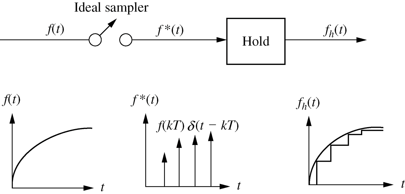
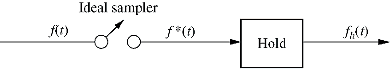
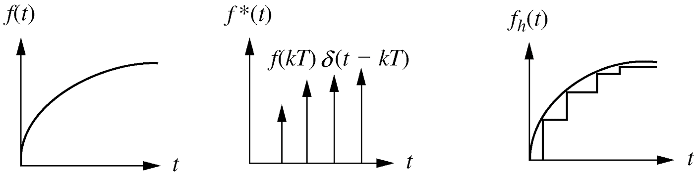
- Sample and zero-order hold transfer function
 \begin{align*}
f_{h}(s) &= G_{zoh}(s) f(s)
\end{align*}
\begin{align*}
f_{h}(s) &= G_{zoh}(s) f(s)
\end{align*}
6z-transform
- $z$-transform definition
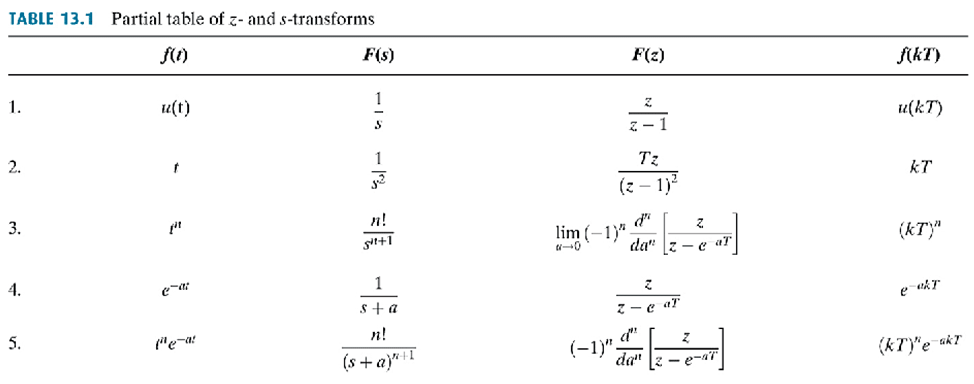
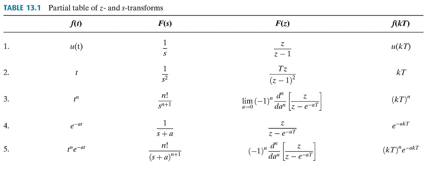
The $z$-transform is defined as: \begin{align*} z &= e^{s\tau} & z^{-1} &= e^{-s\tau} \end{align*} \begin{align*} F(z) &= \mathcal{Z} [F(s)]\\ \end{align*}
Alternatively, the $z$-transform can be calculated from the time domain as an infinite series: \begin{align*} F(z) &= \sum_{k=0}^{\infty} f(k\tau) z^{-k} \end{align*}8- $z$-transform of sample and zero-order hold
\begin{align*} G_{zoh}(s) &= \frac{1-e^{-s\tau}}{s} \\ \\ G_{zoh}(z) &= \mathcal{Z} \left[\frac{1-e^{-s\tau}}{s} \right] \\ \\ &= (1-z^{-1}) \mathcal{Z} \left[ \frac{1}{s} \right] \\ \\ &= \frac{z-1}{z} \mathcal{Z} \left[ \frac{1}{s} \right] \end{align*}1Introduction to digital systems
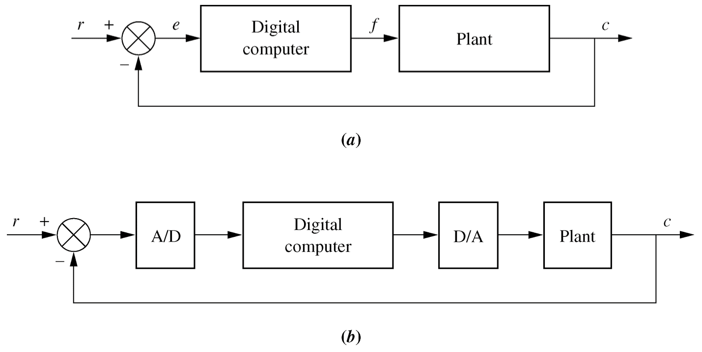
- Analogue to digital, digital to analogue
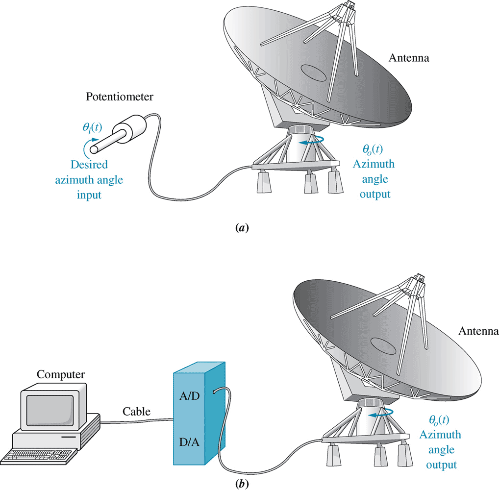
Fig 13.1, p724 / 708, (a) analogue and (b) digital antenna controller5- Sample and zero-order hold transfer function
 \begin{align*}
f_{h}(s) &= G_{zoh}(s) f(s) \\
\\
G_{zoh}(s) &= \frac{1}{s} - \frac{1}{s} e^{-s\tau} = \frac{1-e^{-s\tau}}{s}
\end{align*}
7
\begin{align*}
f_{h}(s) &= G_{zoh}(s) f(s) \\
\\
G_{zoh}(s) &= \frac{1}{s} - \frac{1}{s} e^{-s\tau} = \frac{1-e^{-s\tau}}{s}
\end{align*}
7- Physical interpretation
The $z$ operator shifts back and forth through time. \begin{align*} z^{-2} X &= X(t-2\tau) &=& X_{k-2} \\ \\ z^{-1} X &= X(t-\tau) &=& X_{k-1} \\ \\ ~~ X &= X(t) &=& X_{k} \\ \\ z^{1} X &= X(t+\tau) &=& X_{k+1} \\ \\ z^{2} X &= X(t+2\tau) &=& X_{k+2} \end{align*}9- $z$-transform of a transfer function
Given a continuous transfer function $G(s)$, the digital transfer function $G(z)$ can be calculated by including a ZOH: \begin{align*} G(z) &= \frac{z-1}{z} \mathcal{Z} \left[ \frac{G(s)}{s} \right] \end{align*}
The $z$-transform of $\displaystyle \frac{G(s)}{s}$ can be calculated using tables.
- Sample and zero-order hold transfer function
-
12
- Mapping $s$ to $z$: the origin
Consider the origin of the $s$-domain: \begin{align*} s &=0 \end{align*}
Mapping the origin to the $z$=domain: \begin{align*} z &= e^{s\tau} = e^{0\tau} = 1 \end{align*}14- Mapping $s$ to $z$: the imaginary axis
The imaginary axis in the $s$-domain maps to a unit circle in the $z$-plane: \begin{align*} s &= \pm j\omega & z &= e^{s\tau} = e^{j\omega\tau} \\ &&&= \cos \omega\tau + j \sin \omega\tau \\ &&&= 1 \angle \omega\tau \end{align*} \begin{array}{|c|c|c|c|} \hline \omega\tau & \cos \omega\tau & \sin \omega\tau & z \\ \hline 0 & 1 & 0 & 1 \\ +\frac{\pi}{2} & 0 & 1 & j \\ \pi & -1 & 0 & -1 \\ -\frac{\pi}{2} & 0 & -1 & -j \\ \hline \end{array}16Transfer functions
- Causal digital transfer functions
If the order of the denominator of a transfer function is greater than or equal to the order of the numerator, the system is causal. \begin{align*} G(z) = \frac{y}{u}(z) &= \frac{1}{z+1} \\ \\ (z+1) y &= u \\ \\ y_{k+1} + y_k &= u_k \\ \\ y_{k+1} &= u_k - y_k \end{align*} The next output depends on the current (or past) inputs and outputs.18- Exact analytical transformation
A continuous transfer function $G(s)$ can be converted into a digital transfer function $G(z)$. The digital transfer function depends on the sampling period $\tau$. If the sampling period changes, $G(z)$ must be recalculated.
The transformation can be performed using tables of Laplace transforms, or by using the Matlab (or Octave) command c2d.
Digital transfer functions can also be converted back to the $s$ domain similarly, using tables of transforms or the d2c command.
For a plant, use the 'zoh' method; for a controller, use 'tustin'.20- Plant conversion using c2d
octave:1> gs = zpk( [] , [ -1, -2 ] , 1 )
Transfer function 'gs' from input 'u1' to output ...
            1
 y1:  -------------
      s^2 + 3 s + 2
Continuous-time model.
octave:2 > gz = c2d( gs , 1 , 'zoh' )
Transfer function 'gz' from input 'u1' to output ...
         0.1998 z + 0.0735
 y1:  ------------------------
      z^2 - 0.5032 z + 0.04979
Sampling time: 1 s
Discrete-time model.
13- Mapping $s$ to $z$: the negative real axis
Consider a point on the negative real axis: \begin{align*} s &= -\sigma \end{align*}This maps to the region $0 < z < 1$:\begin{align*} z &= e^{-\sigma \tau} & \qquad \tau & \gt 0 \end{align*} \begin{array}{|l|l|} \hline s & z \\ \hline -0 & 1 \\ -0.5 & 0.60653 \\ -1 & 0.36788 \\ -2 & 0.13534 \\ -\infty & 0 \\ \hline \end{array}15- Mapping $s$ to $z$: general
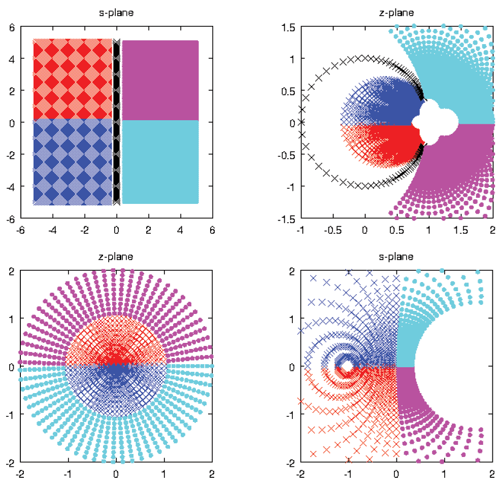
\begin{align*} s &= \sigma + j\omega \\ \\ z &= e^{(\sigma+j\omega)\tau} \\ \\ &= e^{\sigma\tau}e^{j\omega\tau} \\ \\ &= e^{\sigma\tau} (\cos\omega\tau + j\sin\omega\tau) \\ \\ &= e^{\sigma\tau} \angle \omega\tau \end{align*} Note that the position depends on the sampling period $\tau$.17- Non-causal digital transfer functions
If the order of the numerator is greater than the order of the denominator of a transfer function, the system is non-causal. \begin{align*} G(z) = \frac{y}{u}(z) &= \frac{z+1}{1} \\ \\ y &= (z+1) u \\ \\ y_k &= u_{k+1} + u_k \\ \end{align*} The output depends on the future input!19- Example: Exact analytical transformation
[ See Full Equation Here ]\begin{align*} G(z) &= \frac{0.5 \require{cancel} \cancel{(z-1)}}{\cancel{z-1}} - \frac{z-1}{z-e^{-\tau}} + \frac{0.5(z-1)}{z-e^{-2\tau}} \\ \\ \\ \\ &= \frac{ \begin{aligned} 0.5~~&(z-e^{-\tau})&&(z-e^{-2\tau})\\ &&&- (z-1)&&(z-e^{-2\tau}) \\ &&&&&+ 0.5~~(z-1)&&(z-e^{-\tau}) \end{aligned} } {(z-e^{-\tau})(z-e^{-2\tau})} \end{align*}Example: Exact analytical transformation
\begin{align*} G(z) &= \frac{0.5 \require{cancel} \cancel{(z-1)}}{\cancel{z-1}} - \frac{z-1}{z-e^{-\tau}} + \frac{0.5(z-1)}{z-e^{-2\tau}} \\ \\ \\ \\ &= \frac{ \begin{aligned} 0.5~~&(z-e^{-\tau})&&(z-e^{-2\tau})\\ &&&- (z-1)&&(z-e^{-2\tau}) \\ &&&&&+ 0.5~~(z-1)&&(z-e^{-\tau}) \end{aligned} } {(z-e^{-\tau})(z-e^{-2\tau})} \end{align*}
\begin{align*} G(z) &= \frac{ \begin{aligned} 0.5 &( &z^2& - &(& e^{-\tau} &+& e^{-2\tau} &)& &z& &+& e^{-\tau}e^{-2\tau} &)\\ - &( &z^2& - &(& 1 &+& e^{-2\tau} &)& &z& &+& e^{-2\tau} &)\\ + 0.5 &(& z^2& - &(&1 &+& e^{-\tau}&)& &z& &+& e^{-\tau} &) \end{aligned} } { ( z-e^{-\tau} ) ( z-e^{-2\tau} ) } \\ \end{align*}
\begin{align*} G(z) &= \frac{ (0.5-e^{-\tau}+0.5e^{-2\tau}) z + 0.5e^{-\tau}-e^{-2\tau}+0.5e^{-3\tau} } { ( z-e^{-\tau} ) ( z-e^{-2\tau} ) } \end{align*}
\begin{align*} G(z) &= \frac{ \begin{aligned} 0.5 &( &z^2& - &(& e^{-\tau} &+& e^{-2\tau} &)& &z& &+& e^{-\tau}e^{-2\tau} &)\\ - &( &z^2& - &(& 1 &+& e^{-2\tau} &)& &z& &+& e^{-2\tau} &)\\ + 0.5 &(& z^2& - &(&1 &+& e^{-\tau}&)& &z& &+& e^{-\tau} &) \end{aligned} } { ( z-e^{-\tau} ) ( z-e^{-2\tau} ) } \\ \end{align*}
\begin{align*} G(z) &= \frac{ (0.5-e^{-\tau}+0.5e^{-2\tau}) z + 0.5e^{-\tau}-e^{-2\tau}+0.5e^{-3\tau} } { ( z-e^{-\tau} ) ( z-e^{-2\tau} ) } \end{align*} - Mapping $s$ to $z$: the origin
-
22
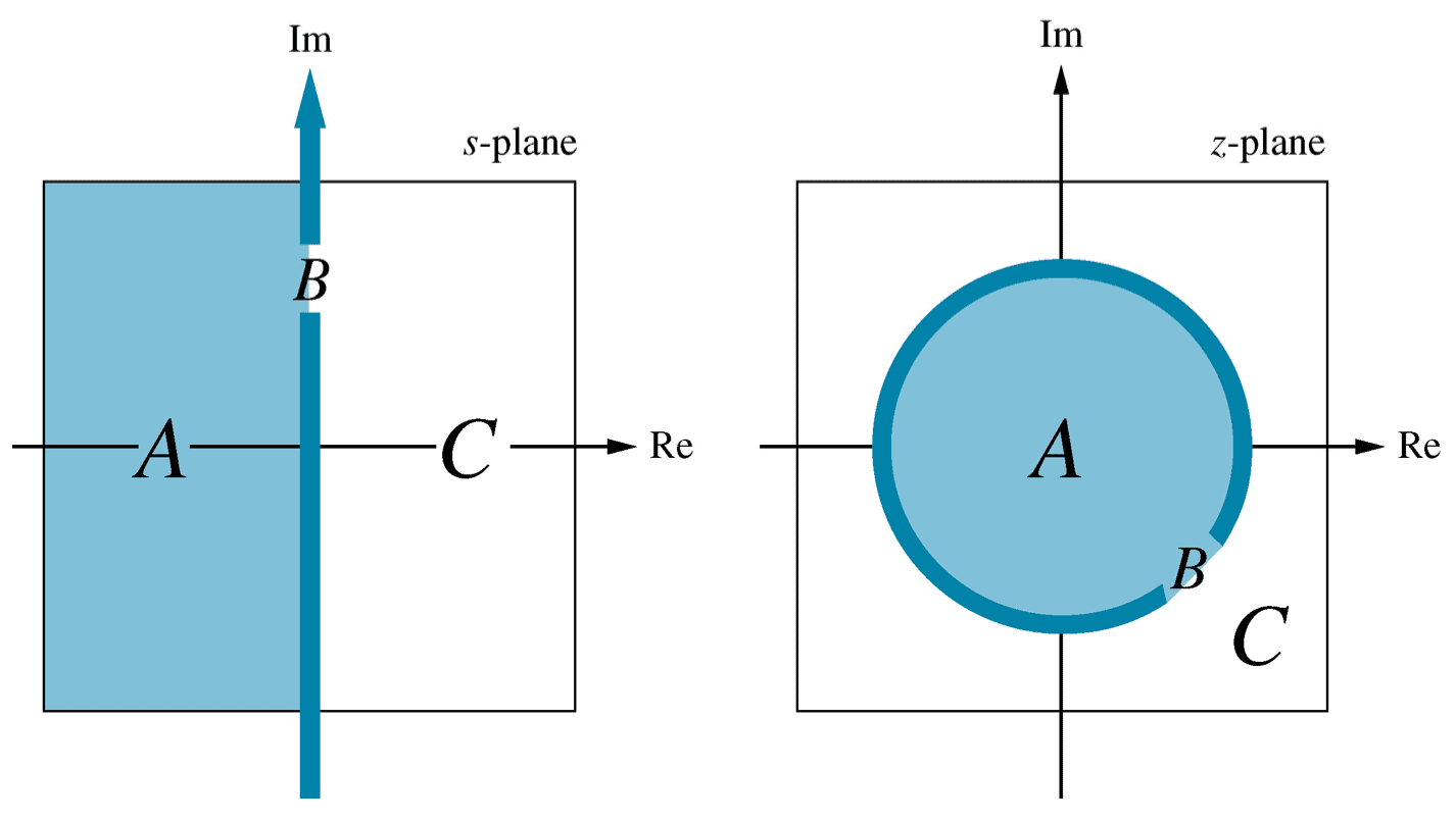
- Pole location
In the $s$-domain, it is required that all poles lie in the left half plane for a system to be stable, i.e.: \begin{align*} Re(s) & \lt 0 \end{align*} In the $z$-domain, we require that all poles lie within the unit circle: \begin{align*} |z| & \lt 1 \end{align*} If all parameters are known, testing that all poles lie within the unit circle is usually the easiest way of testing a system's stability.24- Approximating the $s$ to $z$ mapping
\begin{align*} z &= e^{s\tau} \end{align*} Recall that the exponential function can be expressed as an infinite power series. \begin{align*} e^{s\tau} &= 1 + s\tau + \frac{(s\tau)^2}{2!} + \frac{(s\tau)^3}{3!} + \cdots \end{align*} Various approximations to the true function can be generated.28- Verification code: step response
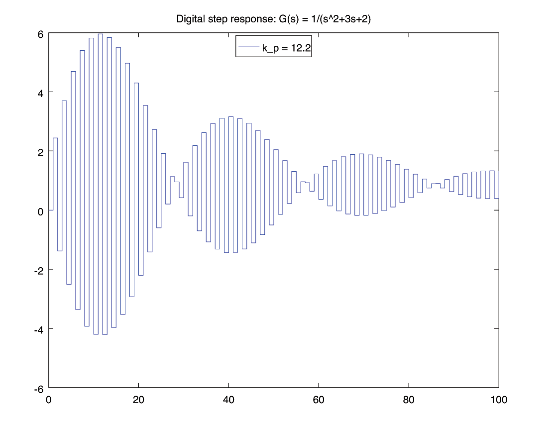
% -*-octave-*-
gs = zpk( [], [-1,-2], 1);
Ts = 1;
gz = c2d( gs, Ts );
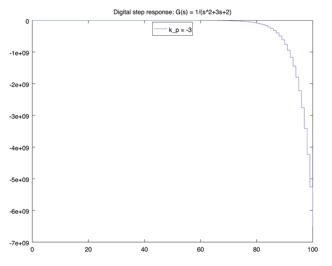
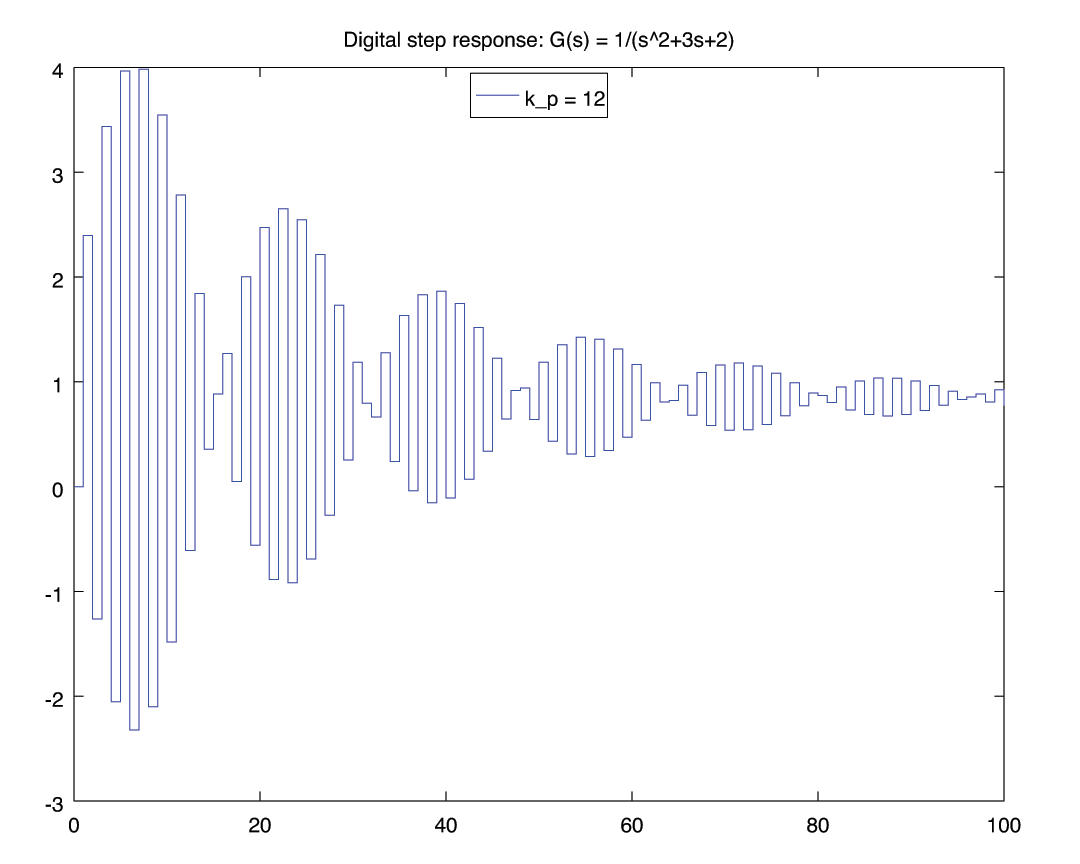
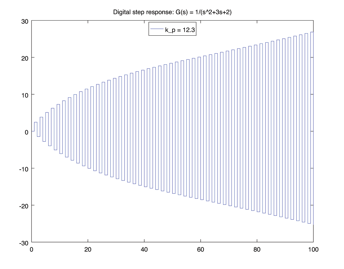
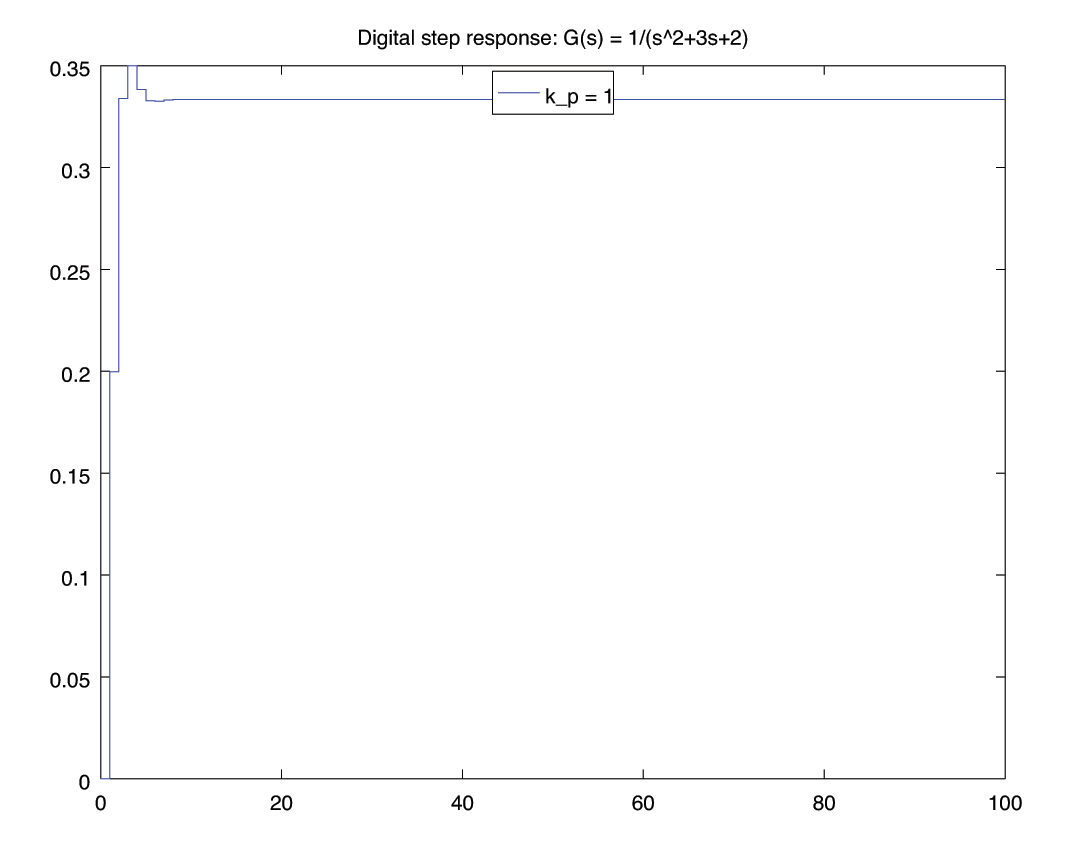
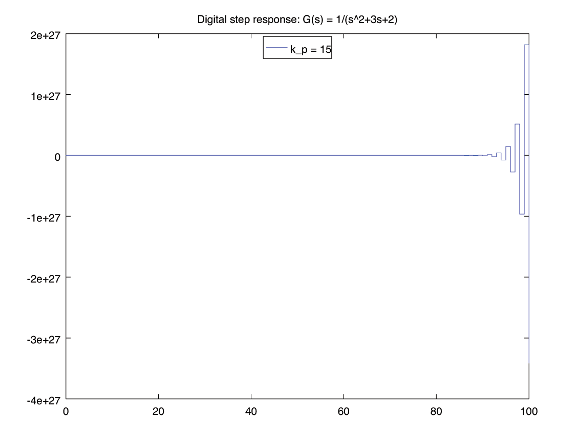
for kp = [ -3, -2, -1 , 1 , 12, 12.2 , 12.3, 15 ]
[y,t] = lsim( feedback(kp*gz, 1), ones(101,1) , 100*Ts);
figure();
stairs(t, y);
legend(['k_p = ', num2str(kp) ], "location", "north");
title('Digital step response: G(s) = 1/(s^2+3s+2)');
print('-depsc', ['stability-k=', num2str(kp), '.eps'])
end23- Routh-Hurwitz
If there are unknown controller parameters, in the $s$-domain we can use the Routh-Hurwitz criteria to determine parametric constraints for stability.
The Routh-Hurwitz criteria do not apply for digital systems. If we wish to analyse a system using the Routh-Hurwitz criteria, we must map it back from the $z$-domain to the $s$-plane.
But a full mapping from $z$ to $s$ is not always simple when there are unknown parameters.25- A bilinear transform
A bilinear transform is a transformation that is linear in both directions: $s$ to $z$ and $z$ to $s$.
The following bilinear transform is not a faithful mapping between $s$ and $z$, but does map the left half plane of $s$ to the unit circle of $z$. Thus it can be used for stability analysis. \begin{align*} s &= \frac{z+1}{z-1} & z &= \frac{s+1}{s-1} \end{align*} Given a digital transfer function $G(z)$, we can substitute $z$ to get an $s$-domain approximation which can be analysed for stability using the Routh-Hurwitz criteria.
Note that this mapping does not include the system sampling period $\tau$. It therefore does not faithfully preserve transient behaviour and frequency response characteristics.27- Example: P control of G(z)
Example: $L=1$ H, $R=20 \Omega$, $C=0.01$ F. % s=-10
Consider digital proportional control of plant $G(s)$ with sampling period $\tau = 1$ s. \begin{align*} G(s) &= \frac{1}{(s+1)(s+2)} \\ \\ G(z) &= \frac{0.1998 z + 0.0735}{z^2 - 0.5032 + 0.04979} & \text{Use c2d} \\ \end{align*} Find the range of gains $k_p$ for stability, using Routh Hurwitz. \begin{align*} K(z) &= k_p \\ \\ T(z) &= \frac{K(z)G(z)}{1+K(z)G(z)} \end{align*}
To apply RH, first transform back to the $s$ domain. \begin{align*} T(z) &= \frac{19980 \,k_p z + 7350 \,k_p}{100000 z^2 + 740 (27 \,k_p - 68) z + (7350 \,k_p+4979)} \end{align*} Stability analysis, $\therefore$ can use simple bilinear transform \begin{align*} z &= \frac{s+1}{s-1} \end{align*} Substitute into $T(z)$ to get $T(s)$. \begin{align*} T(s) &= \frac{19980 \,k_p \frac{s+1}{s-1} + 7350 \,k_p}{100000 \left(\frac{s+1}{s-1}\right)^2 + 740 (27 \,k_p - 68) \frac{s+1}{s-1} + (7350\,k_p+4979)} \\ \\ &= \frac{27330 s^2 - 14700 \,k_p s - 12630 \,k_p}{(27330 \,k_p+54659) s^2 + 2(95021-7350\,k_p) s + (155299-12630 \,k_p)} \end{align*}
Apply Routh-Hurwitz criteria \begin{align*} T(s) &= \frac{27330 s^2 - 14700 \,k_p s - 12630 \,k_p}{(27330 \,k_p+54659) s^2 + 2(95021-7350\,k_p) s + (155299 - 12630 \,k_p)} \end{align*} \begin{align*} \text{R-H 1:}\qquad k_p &\neq -\frac{54659}{27330} &\text{~and~} k_p &\neq \frac{95021}{7350} &\text{~and~} k_p &\neq \frac{155299}{12630} \\ \\ \text{R-H 2:}\qquad k_p & \gt -\frac{54659}{27330} &\text{~and~} k_p & \lt \frac{95021}{7350} &\text{~and~} k_p & \lt \frac{155299}{12630} \\ \end{align*} Routh array: \begin{align*} \begin{matrix} s^2 &:& 27330 \,k_p + 54659 & 155299 - 12630 \,k_p \\ s^1 &:& 2(95021 - 7350 \,k_p) & 0 \\ s^0 &:& b_1 & \end{matrix} \end{align*}
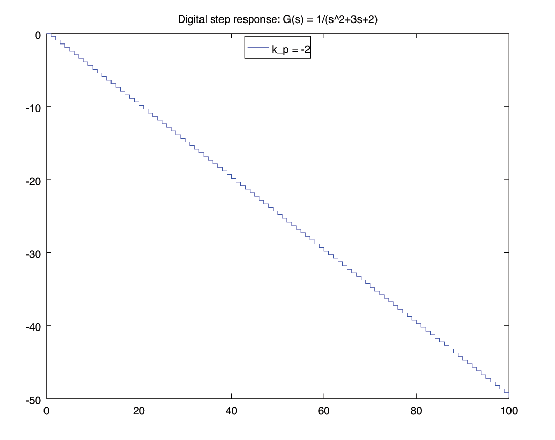
R-H 3: \begin{align*} \begin{matrix} s^2 &:& 27330 \,k_p + 54659 & 155299 - 12630 \,k_p \\ s^1 &:& 2(95021 - 7350 \,k_p) & 0 \\ s^0 &:& b_1 & 0 \end{matrix} \end{align*} \begin{align*} b_1 &= \frac{\left| \begin{matrix} 27330 \,k_p + 54659 & 155299 - 12630 \,k_p\\ 2(95021 - 7350 \,k_p) & 0 \\ \end{matrix} \right|}{- 2(95021-7350 \,k_p)} \\ &= 12630 \,k_p - 155299 \end{align*} \begin{align*} \begin{matrix} s^2 &:& 27330 \,k_p + 54659 & \gt 0 & \implies & k_p &\gt& -2 \\ s^1 &:& 2(95021 - 7350 \,k_p) & \gt 0 & \implies & k_p & \lt & 12.928\\ s^0 &:& 12630 \,k_p - 155299 & \gt 0 & \implies & k_p & \lt & 12.296 \end{matrix} \end{align*} \begin{align*} -2 \lt k_p \lt 12.296 \end{align*}
- Pole location
-
36
Steady state errors
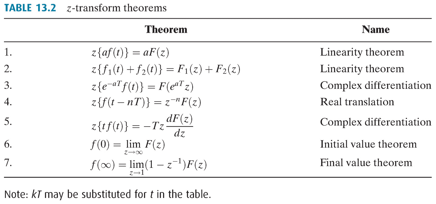
- Final value theorem
Just as there is a final value theorem in the $s$-domain: \begin{align*} F(\infty) &= \lim_{s\rightarrow 0} s F(s) \end{align*} There is an equivalent final value theorem in the $z$-domain: \begin{align*} F(\infty) &= \lim_{z\rightarrow 1} (1-z^{-1}) F(z) \\ \\ &= \lim_{z\rightarrow 1} \frac{z-1}{z} F(z) \end{align*}37- Static error constants
In Chapter 7, static error constants were derived for various inputs in the $s$-domain. Equivalent constants can be derived in the $z$-plane (p750 / 734).
Unit step input \begin{align*} K_p &= \lim_{z\rightarrow 1} G(z) & e(\infty) &= \frac{1}{1+K_p} \end{align*} Unit ramp input \begin{align*} K_v &= \lim_{z\rightarrow 1} (z-1) G(z) & e(\infty) &= \frac{1}{K_v} \end{align*} Unit parabolic input \begin{align*} K_a &= \frac{1}{\tau^2} \lim_{z\rightarrow 1} (z-1)^2 G(z) & e(\infty) &= \frac{1}{K_a} \end{align*} - Final value theorem
-
41
- Tustin transform of a PID controller
Find the digital transfer function of a PID controller using Tustin. \begin{align*} K(s) &= K_P + \frac{K_I}{s} + K_Ds \\ \end{align*} Substitute the Tustin transform for $s$ \begin{align*} s &= \frac{2(z-1)}{\tau(z+1)} \\ \\ K(z) &= K_P + \frac{K_I}{\frac{2(z-1)}{\tau(z+1)}}+K_d\frac{2(z-1)}{\tau(z+1)} \end{align*} Then rearrange into a useful form.
\begin{align*} K(z) &= K_P + \frac{K_I}{\frac{2(z-1)}{\tau(z+1)}}+K_d\frac{2(z-1)}{\tau(z+1)} \\ \\ \\ &= K_P + \frac{K_I\tau(z+1)}{2(z-1)} + K_d\frac{2(z-1)}{\tau(z+1)} \\ \\ \\ &= \frac{K_P(2\tau(z-1)(z+1)+K_I\tau^2(z+1)^2+K_D2^2(z-1)^2}{2\tau(z-1)(z+2)} \end{align*}43- Summary
- When in doubt, use the exact transform.
- Do not forget the ZOH when converting a plant.
- Use Tustin when converting a digital controller.
- Use the simple bilinear transform only for stability analysis.
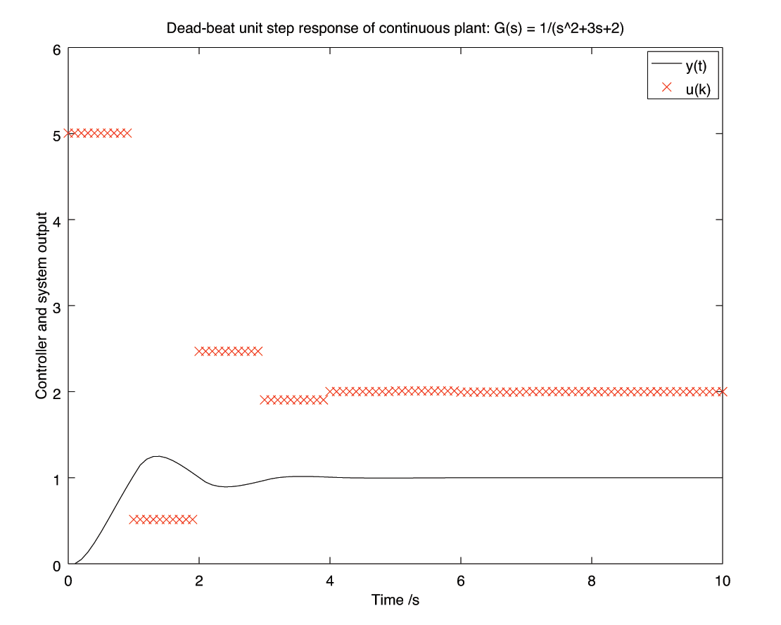
45- Dead-beat control method: $y_k = r_{k-1}$
\begin{align*} T(z) &= \frac{ K(z) G(z) } { 1+K(z)G(z) } \; \;\text{Require~} T(z) = z^{-1} \\ \\ K(z)G(z) &= z^{-1} \left( 1+K(z)G(z) \right) \; \;\text{Divide all by $G(z)$} \\ \\ (1-z^{-1}) K(z) &= z^{-1} G^{-1} \;\; \text{Multiply all by $z$}\\ \\ K(z) &= \frac{1}{(z-1)G(z)} \end{align*}47- Dead-beat controller
\begin{align*} G(s) &= \frac{1}{(s+1)(s+2)} \\ \\ G(z) &= \frac{0.1998 z + 0.0735}{z^2 - 0.5032 z + 0.04979} \\ \\ K(z) &= \frac{z^2 - 0.5032 z + 0.04979}{0.1998z^2 - 0.1263 z - 0.0735} \\ \\ T(z) &= \frac{K(z)G(z)}{1+K(z)G(z)} \\ \\ &= \frac{0.1998 z^3 - 0.02704 z^2 - 0.02704 z + 0.003659} {0.1998 z^4 - 0.02704 z^3 - 0.02704 z^2 + 0.003659 z} \end{align*}
\begin{align*} K(z) = \frac{u}{e}(z) &= \frac{z^2 - 0.5032 z + 0.04979}{0.1998z^2 - 0.1263 z - 0.0735} \\ \end{align*}
\begin{align*} (0.1998 z^2 - 0.1263 z - 0.0735) \,u &= (z^2 - 0.5032 z + 0.04979) \,e \\ \\ 0.1998 \,u_{k+2} - 0.1263 \,u_{k+1} - 0.0735 \,u_k &= e_{k+2} - 0.5032 \,e_{k+1} + 0.04979 \,e_{k} \\ \\ 0.1998 \,u_{k} - 0.1263 \,u_{k-1} - 0.0735 \,u_{k-2} &= \,e_{k} - 0.5032 \,e_{k-1} + 0.04979 \,e_{k-2} \\ \end{align*} \begin{align*} u_k &= e_{k} - \frac{0.5032}{0.1998} e_{k-1} - \frac{0.04979}{0.1998} e_{k-2} + \frac{0.1263}{0.1998} u_{k-1} + \frac{0.0735}{0.1998} u_{k-2} \\ \\ u_k &= -2.5182 \,e_{k} - 0.24920 \,e_{k-1} + 0.63213 \,u_{k-1} + 0.36787 \,u_{k-2} \end{align*}38Transient response
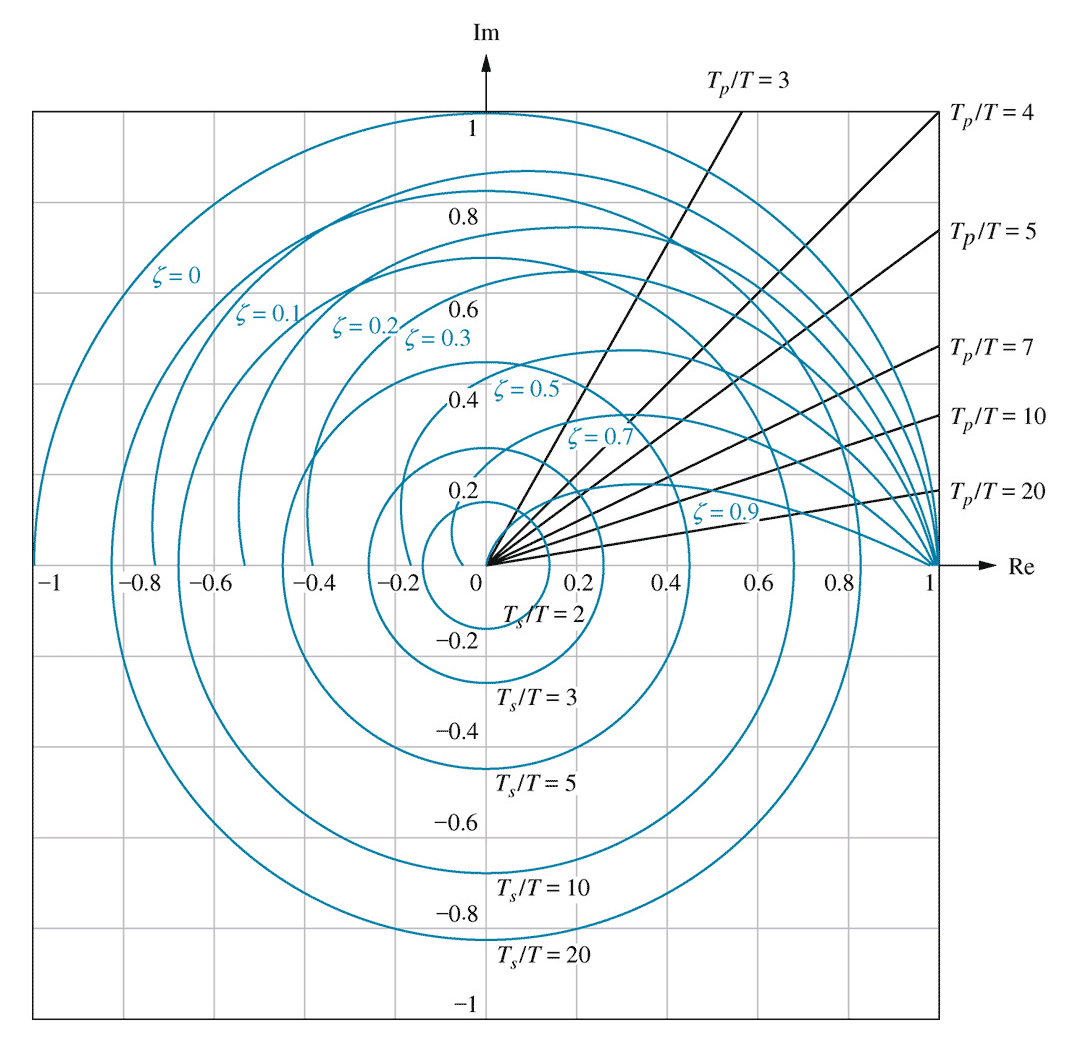
- Transient response on the $z$-plane
Digital controllers are commonly designed on the $s$-plane to give desired performance and then converted into digital controllers using the $z$-transform.
However, it is possible to undertake pole placement on the $z$-plane directly.40Cascade compensation on the z-plane
- The Tustin transformation
The Tustin transformation is a mapping between the $s$ and $z$-planes that preserves frequency behaviour at the sampling points. Thus it can be used to convert a controller from the $s$-plane into the $z$-domain, and vice versa.
\begin{align*} s &= \frac{2(z-1)}{\tau(z+1)} & z &= \frac{-\left(s+\frac{2}{\tau}\right)}{\left(s-\frac{2}{\tau}\right)} = \frac{1+\frac{\tau}{2}s}{1-\frac{\tau}{2}s} \end{align*}
Note that the Tustin transform depends on the sampling period $\tau$. Changing the sampling period requires the controller to be recalculated.42- Tustin transform of PID using Reduce
$ reduce
Reduce (Free PSL version), 4-Sep-2014 ...
1: k := Kp + Ki/s + Kd*s ;
          2
      kd*s  + ki + kp*s
k := -------------------
              s
2: s := 2*(z-1) / ( T*(z+1) ) ;
      2*(z - 1)
s := -----------
      t*(z + 1)
3: factor z ;
4: k;2 2 2 2 z *(4*kd + ki*t + 2*kp*t) + 2*z*( - 4*kd + ki*t ) + 4*kd + ki*t - 2*kp*t ---------------------------------------------------------------------------- 2 2*z *t - 2*t44Design: Dead beat
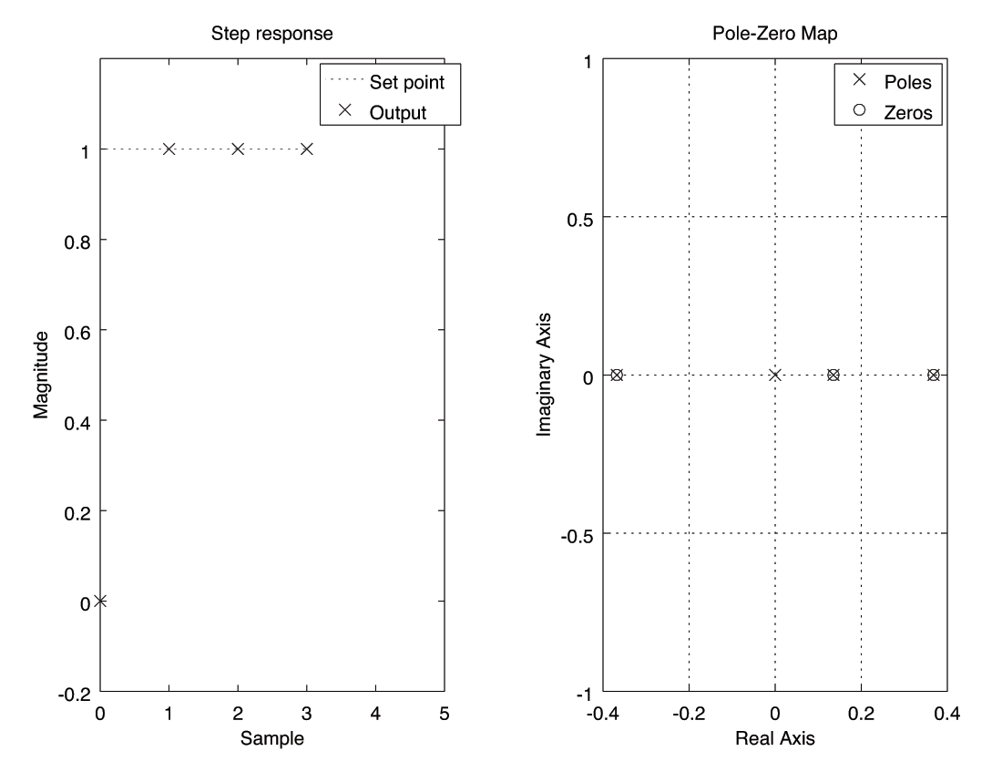
- Dead-beat control
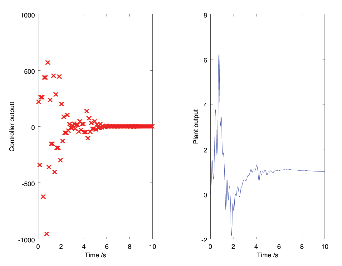
Digital control enables a range of interesting control methods to be implemented. An example is dead-beat control, where the output is forced to achieve a set-point reference in a minimum number of samples. This is achieved by designing a controller such that the closed loop transfer function is: \begin{align*} T(z) &= z^{-1} \end{align*} In practice, dead-beat controllers tend to require very large controller outputs.
Design a dead-beat controller for the plant: \begin{align*} G(s) &= \frac{1}{(s+1)(s+2)} \end{align*}
46- Dead-beat control design with Matlab or Octave
% -*-octave-*-
clear all
gs = zpk( [], [-1,-2 ], 1 ) % continuous plant
Ts = 1 % sampling period [s]
gz = c2d( gs, Ts, 'zoh' ) % digital plant
z = tf('z', Ts) % z operator
k = 1/(gz*(z-1)) % dead-beat controller
T = feedback(k*gz,1) % closed loop transfer function
n = 4 % number of samples to simulate
r = ones(n,1) % set point reference input
[y,t,x] = lsim(T, r, (n-1)*Ts) % simulation
- Tustin transform of a PID controller
-
51
- Code for digital design and continuous simulation
% -*-octave-*- clear all; % continuous plant specification: 2 real poles gs = zpk( [], [-1,-2], 1); % convert to continuous state space model for simulation [A,B,C,D] = tf2ss(gs); % design digital controller Ts = 1; % sampling period [s] gz = c2d( gs, Ts); % convert plant to digital (zoh) z = tf('z', Ts); % z operator T = 1/z; % dead-beat controller target kz = T/(gz*(1-T)) % control design! % Control law will be of the form: % u_k = Kb(1)*e_k + Kb(2)*e_{k-1} ... - Ka(1)*u_{k-1} - Ka(2)*u_{k-2} ... % copy controller coefficients into matrices for implementation [b,a] = ss2tf(ss(kz)) % get coefficients of controller Kb = zeros(1,10); % initialise arrays to zero Ka = zeros(1,10); % (10 elements is larger than needed) Kb(1:length(b)) = b./a(1); % populate with controller coefficients Ka(1:length(a)-1) = a(2:end)./a(1); % initialise past I/O signals to zero ez = zeros(size(Ka')); uz = zeros(size(Kb')); % initialise plant and set point x = zeros(size(A,1),1); % zero all states (number from state matrix) u0 = 0; % zero controller output ref = 1; % set-point reference % simulation parameters dt = 0.1; % simulation step size t1 = 10; % simulation end time % initialise data record (more efficient than dynamic memory reallocation) data = zeros(t1*dt+1, 3); % number of sample times, [t,u,y] row = 0; % counter for inserting data records for t = 0.0 : dt : t1 % loop over time row = row + 1; y = C*x + D*u0; % update outputs (continuous) % if at sampling time ... if (mod(t,Ts) == 0) % update error and control output disp('Sampling:'), t e0 = ref-y; % measure current error ez = shift(ez,1); % shift old errors by 1 sample ez(1) = e0; % update register with current error u0 = Kb*ez - Ka*uz; % compute control output! uz = shift(uz,1); % shift old inputs back 1 sample uz(1) = u0; % update register with current output end % update plant every step xdot = A*x + B*u0; % update rates using last held input x = x + xdot*dt; % Forward Euler integration data(row,:) = [t,u0,y]; % save data (continuous) end t = data(:,1); u = data(:,2); y = data(:,3); figure(2); plot(t,y ,'-k', t,u,'xr'); legend({'y(t)','u(k)'}) title('Dead-beat unit step response of continuous plant: G(s) = 1/(s^2+3s+2)') xlabel('Time /s'); ylabel('Controller and system output'); print -depsc 'deadbeat-continuous.eps'48- Dead-beat control design with Matlab or Octave
figure(1) % new window subplot(121) % subfigure 1x2 plot 1 plot(t,r,'r:',t,y,'bx') % plot data axis([0,5,-0.2,1.2]) % fix axis range title('Step response') % chart title xlabel('Sample') % axis label ylabel('Magnitude') % axis label legend({'Set point','Output'}) % chart key subplot(122) % subfigure 1x2 plot 2 pzmap(T) % pole zero map legend({'Poles','Zeros'}) % chart key print -deps 'deadbeat.eps' % print using eps format - Code for digital design and continuous simulation
-
54
Design: IMC
- Internal model control
A similar approach to direct synthesis is to factor the open-loop plant as: \begin{align*} G &= G_{P^+} G_{P^-} \end{align*} where $G_{P^+}$ contains any time delays or zeros outside the stable region. A controller $K$ is then defined using an inverse of only the part $G_{P^-}$ which will not give rise to unstable controller poles. \begin{align*} K &= \frac{1}{G_{P^-}} f \end{align*} where $f$ is a low pass filter with a steady gain of 1.56- Digital state space poles
The poles of a digital state space system are the eigenvalues of the digital state matrix $\mathrm{F}$: \begin{align*} \left| z \mathrm{I} - \mathrm{F} \right| &= 0 \end{align*} Compare to a continuous system: \begin{align*} \left| s \mathrm{I} - \mathrm{A} \right| &= 0 \end{align*}58- Digital pole placement (MIMO)
\begin{align*} \begin{pmatrix} \underset{\sim}{x} \\ \underset{\sim}{x}_{N} \end{pmatrix}_{k+1} &= \begin{pmatrix} \mathrm{F}-\mathrm{G}\mathrm{K} & \mathrm{G}\mathrm{k_e} \\ -\mathrm{H} & \mathrm{I} \end{pmatrix} \begin{pmatrix} \underset{\sim}{x} \\ \underset{\sim}{x}_{N} \end{pmatrix}_k + \begin{pmatrix} \mathrm{0} \\ \mathrm{I} \end{pmatrix} \begin{pmatrix} \underset{\sim}{r} \end{pmatrix}_{k+1} \end{align*} And the controlled system closed loop poles are at: \begin{align*} \left| z\mathrm{I} - \mathrm{F}^* \right| &= 0 & \mathrm{F}^* &= \begin{pmatrix} \mathrm{F}-\mathrm{G}\mathrm{K} & \mathrm{G}\mathrm{k_e} \\ -\mathrm{H} & \mathrm{I} \end{pmatrix} \end{align*}
53Design: Synthesis
- Direct synthesis
The dead-beat controller created previously was designed using the method of direct synthesis. For a unity feedback control system: \begin{align*} T(s) &= \frac{K(s)G(s)}{1+K(s)G(s)} \;\; \rightarrow \;\; K(s) = \frac{T(s)}{G(s)(1-T(s))} \\ \\ T(z) &= \frac{K(z)G(z)}{1+K(z)G(z)} \;\; \rightarrow \;\; K(z) = \frac{T(z)}{G(z)(1-T(z))} \end{align*} Thus if a target closed-loop transfer function $T(s)$ or $T(z)$ is defined, and the open-loop plant model $G(s)$ or $G(z)$ is known, the controller $K(s)$ or $K(z)$ can be computed directly.
\begin{align*} K &= \frac{T}{G(1-T)} \end{align*} Direct synthesis relies on pole-zero cancellation to suppress unwanted dynamics, based on an inverse model of the plant, i.e. $G^{-1}(s)$ or $G^{-1}(z)$.
Model inversion means that any non-minimum phase zeros (outside the stable region) in the plant will become unstable poles in the controller.
If the model parameters do not exactly match the real world (and they won't), the pole-zero cancellation will not be exact and unwanted dynamics will occur.
This method does not guarantee that the controller will be physically realisable. That must be checked before use.55Design: Placement
- Pole placement
Pole placement can be used in the digital domain directly. It is necessary to first consider the digital state space representation.
Whereas a continuous state space model uses ordinary differential equations a digital state space model is defined by difference equations. \begin{align*} \underset{\sim}{\dot x} &= \mathrm{A} \underset{\sim}{x} + \mathrm{B} \underset{\sim}{u} & \underset{\sim}{y} &= \mathrm{C} \underset{\sim}{x} \\ \underset{\sim}{x}_{k+1} &= \mathrm{F} \underset{\sim}{x}_k + \mathrm{G} \underset{\sim}{u}_{k+1} & \underset{\sim}{y}_{k+1} &= \mathrm{H} \underset{\sim}{x}_k \end{align*} Use c2d() to convert from continuous to discrete.57- Pole placement with integral action
Using an identical structure to that used for continuous pole placement (p.700 / p.684) and noting that an integrator in the $z$ domain is: \begin{align*} \frac{1}{s} &\leftrightarrow \frac{z}{z-1} &\implies& \frac{x_N}{e}(z) = \frac{z}{z-1} \end{align*} Thus integral action gives rise to the following expression: \begin{align*} (z-1) \underset{\sim}{x}_N &= z \underset{\sim}{e} \\ \underset{\sim}{x}_{N,k+1} - \underset{\sim}{x}_{N,k} &= \underset{\sim}{e}_{k+1} \\ \underset{\sim}{x}_{N,k+1} &= \underset{\sim}{x}_{N,k} + \underset{\sim}{e}_{k+1} \\ &= \underset{\sim}{x}_{N,k} + \underset{\sim}{r}_{k+1} - \underset{\sim}{y}_{k+1} \\ &= \underset{\sim}{x}_{N,k} + \underset{\sim}{r}_{k+1} - \mathrm{H} \underset{\sim}{x}_k \end{align*}59Liability
- Limitations of Liability
"LIMITATION OF LIABILITY. The Programs should not be relied on as the sole basis to solve a problem or implement a design whose incorrect solution or implementation could result in injury to person or property. If a Program is employed in such a manner, it is at the Licensee’s own risk and MathWorks and its Licensors explicitly disclaim all liability for such misuse to the extent allowed by law."
- Internal model control