2 An Introduction to Graph Theory

2.1 Introduction

In recent years graph theory has become established as an important area of mathematics and computer science. The origins of graph theory however can be traced back to Swiss mathematician Leonhard Euler and his work on the Königsberg bridges problem (1735), shown schematically in Figure 1.

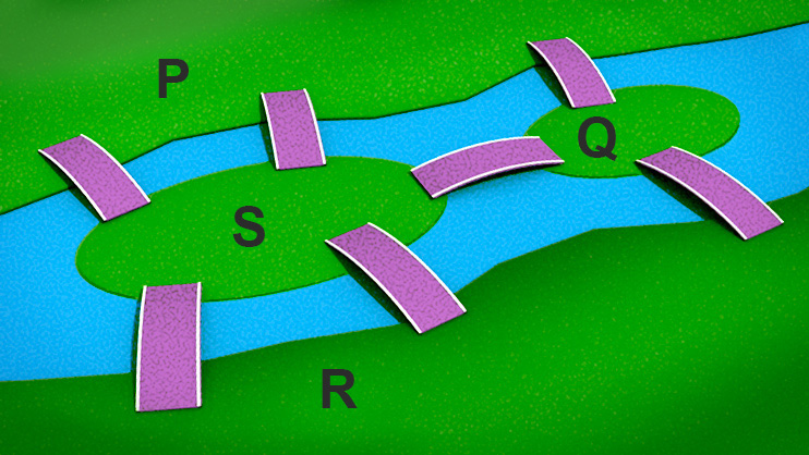
Bridges of Königsberg

Königsberg was a city in 18^th century Germany (it is now called Kaliningrad and is a Russian semi-exclave) through which the river Pregel flowed. The city was built on both banks of the river and on two large islands in the middle of the river. Seven bridges were constructed so that the city’s inhabitants could travel between the four parts of the city; labelled \(P\), \(Q\), \(R\) and \(S\) in the diagram. The people wondered whether or not it was possible for someone to walk around the city in such a way that each bridge was crossed exactly once with the person ending up at their starting point. All attempts to do so ended in failure. In 1735 however Euler presented a solution to the problem by showing that it was impossible to perform such a journey. Euler reasoned that anyone standing on a land mass would need a way to get on and off. Therefore each land mass would require an even number of bridges. In Königsberg each land mass had an odd number of bridges explaining why all seven bridges could not be crossed without crossing one more than once. In formulating his solution Euler simplified the bridge problem by representing each land mass as a point and each bridge as a line as shown in Figure 2.1, leading to the introduction of graph theory and the concept of an Eulerian graph. A closely related problem showed that if the journey started at one land mass and ended at another, crossing each bridge exactly once, then only those two land masses could have an odd number of bridges.

Two other well-known problems from graph theory are:

• Graph Colouring Problem: How many colours do we need to colour a map so that every pair of countries with a shared border have different colours?
• Travelling Salesman Problem: Given a map of several cities and the roads between them, what is the shortest route for a travelling salesman to visit (pass through) each of the cities exactly once?

Some of the applications of graph theory include:

• communication network design
• planning airline flight routes
• using GPS to find the shortest path between two points
• design of electrical circuits
• modelling of the World Wide Web.

2.2 Definitions

The Königsberg bridge problem can be represented diagramatically by means of a set of points and lines. The points \(P\), \(Q\), \(R\) and \(S\) are called vertices, the lines are called edges, and the whole diagram is called a graph.

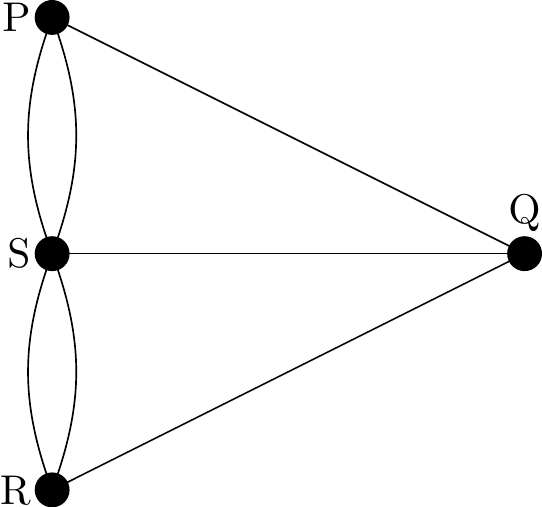
Figure 2.1: Graphical representation of the Königsberg bridge problem

2.2.1 Vertices and Edges

(Very formal definition)

A graph, \(G\), is a mathematical structure which consists of:

• a vertex set \(V = V(G)\) whose elements are called vertices of \(G\)³.
• an edge set \(E = E( G)\) of unordered⁴ pairs of distinct vertices called edges of \(G\). Note that \(E\) is actually a multiset in that some unordered pairs can be repeated to represent more than one edge joining the same two vertices.
• a relation that associates with each edge two vertices, which are not necessarily distinct, called its endpoints.

Such a graph is denoted \(G = \left\{ V( G), E( G) \right\}\), or just simply \(G = \left\{ V, E \right\}\).

Example 1

Consider the graph \(G\) shown in the diagram below.

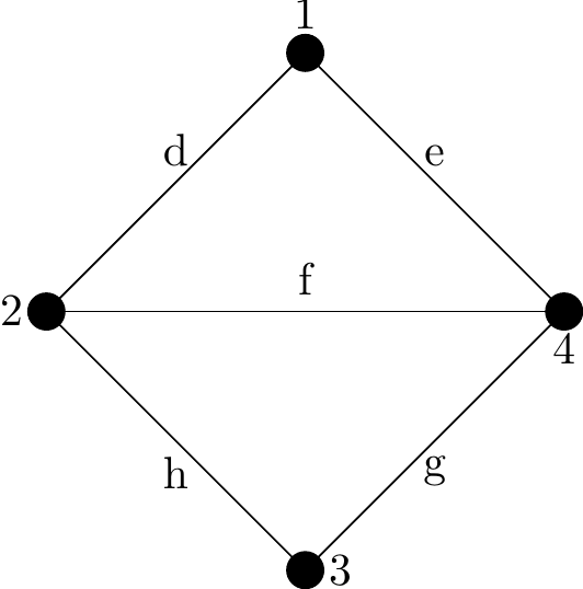
Figure 2.2: Graph with four vertices and five edges

The set \(V\) consists of the four vertices, 1, 2, 3 and 4, i.e. \[ V( G) = \left\{ 1, 2, 3, 4 \right\}.\]

The set \(E\) consists of the five edges, \[ d = \left\{ 1, 2 \right\}, e = \left\{ 1, 4 \right\}, f = \left\{ 2, 4 \right\}, g = \left\{ 3, 4 \right\}, h = \left\{ 2, 3 \right\}\]

i.e. \(E(G) = \left\{ d, e, f, g, h \right\}.\)

Hence, \[ G = \left\{ V( G), E( G) \right\} = \left\{ \left\{ 1, 2, 3, 4 \right\},\left\{ d, e, f, g, h \right\} \right\} \]

Each edge is associated with two vertices called its endpoints.

For example, in Figure 2.2, vertices 1 and 2 are the endpoints of \(d\) and \(d\) is said to connect vertices \(1\) and \(2\).

An edge-endpoint function on a graph \(G\) defines a correspondence between edges and their endpoints.

Example 2

The edge-endpoint function for the graph in Figure 3 is given in the following table:

Edge	Endpoints
d	{ 1, 2 }
\(e\)	{ 1, 4 }
f	{ 2, 4 }
g	{ 3, 4 }
\(H\)	{ 2, 3 }

Now for a couple of new definitions:

Definition of undirected

An undirected graph is a graph in which the edges have no orientation⁵. Hence, in an undirected graph the edge set is composed of unordered vertex pairs⁶. In Figure 2.2 for example, the edge \(\left\{ 1, 2 \right\}\) is considered identical to the edge \(\left\{ 2, 1 \right\}\). This is the principle of unorderedness, the order doesn’t matter.

See later for the definition of directed.

Definition of adjacent and incident

If \(X\) and \(Y\) are vertices of a graph, \(G\), then \(X\) and \(Y\) are said to be adjacent if they are joined by an edge (or more than one edge).

An edge in a graph that joins two vertices is said to be incident to both vertices.

Example 3

We start by redrawing Figure 2.2:

Figure 2.2: Graph with four vertices and five edges

we have the following adjacent vertices:

• vertices 1 and 2 are adjacent
• vertices 1 and 4 are adjacent
• vertices 2 and 3 are adjacent
• vertices 2 and 4 are adjacent
• vertices 3 and 4 are adjacent

The edges that are incident with pairs of vertices as follows:

• edge d is incident to vertices 1 and 2
• edge \(e\) is incident to vertices 1 and 4
• edge f is incident to vertices 2 and 4
• edge g is incident to vertices 3 and 4
• edge \(H\) is incident to vertices 2 and 3

Definition of parallel edges

Two edges connecting the same vertices are called multiple or parallel edges.

These notes are slightly unusual in consider parallel edges at this stage. Many authors do not allow parallel edged and reserve their study for later. In such texts graphs which allow more than one edge to join a pair of vertices are instead called multigraphs.

Example 4

In Figure 2.3 edges \(f\) and \(g\) are parallel edges:

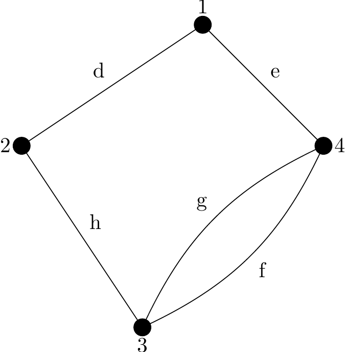
Figure 2.3: A graph containing parallel edges

Now for some final definitions before we can first start to discuss properties of graphs.

Definitions of order, size and degree

The order of a graph, \(G\), denoted \(|V(G)|\), is the number of vertices contained in \(G\).

In Figure 2.3, \(|V(G)| = 4\).

The size of a graph, \(G\), denoted \(| E(G)|\), is the number of edges contained in \(G\).

In Figure 2.3, \(|E(G)| = 5\).

The degree of a vertex \(X\), written \(\mathop{deg}(X)\), is the number of edges in \(G\) that are incident with \(X\).

In Figure 2.3, \(\mathop{deg}(1) = 2\), \(\mathop{deg}(2) = 2\), \(\mathop{deg}( 3) = 3\) and \(\mathop{deg}( 4) = 3\).

Any vertex of degree zero is called an isolated vertex and a vertex of degree one is an end-vertex⁷.

Example 5

In the graph below vertex \(5\) is an isolated vertex and vertex \(3\) is an end-vertex.

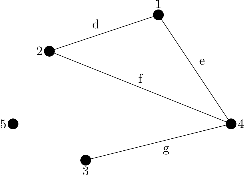
Figure 2.4: A Graph containing an isolated vertex

2.3 The Handshaking Lemma

Definition of odd and even vertices

A vertex is said to be even or odd according to whether its degree is an even or odd number.

So in Figure 2.2, vertices \(2\) and \(4\) are odd while vertices \(1\) and \(3\) are even.

And in Figure 2.4, vertices \(1,2\) and \(5\) are even (with degrees \(2,2,0\) respectively), and vertices \(3\) and \(4\) are odd.

If the degrees of all the vertices in a graph, \(G\), are summed then the result is an even number. Furthermore, this value is twice the number of edges, as each edge contributes 2 to the total degree sum. This result is important enough to be called a lemma, and given a name.

The Handshaking Lemma

In any undirected graph the sum of the vertex degrees is equal to twice the number of edges, i.e.

\[ \sum_{X \in V(G)}{\mathop{deg}( X)} = 2\left| E( G) \right| \]

Proof: In a graph \(G\) an arbitrary edge \(\left\{ X, Y \right\}\) contributes 1 to \(\mathop{deg}( X)\) and 1 to \(\mathop{deg}( Y)\). Hence the degree sum for the graph is even and twice the number of edges.

A corollary of the Handshaking Lemma states that the number of odd vertices in a graph must be even. So, for example, we cannot have a graph with 5 even vertices and 5 odd vertices as the degree sum would be an odd number, contradicting the Handshaking Lemma.

So having defined the degree of a vertex it now turns out that it can be useful to inspect the full list of degrees of a graph to check we haven’t made an error and to get a first idea of what sort of graph it is.

Definition of degree sequence

The degree sequence of an undirected graph \(G\) is a bracketed list of the degrees of all the vertices written in ascending order with repetition as necessary.

Example 6

The degree sequence of the graph in the diagram below is \(( 1, 2, 2, 3, 4 )\).

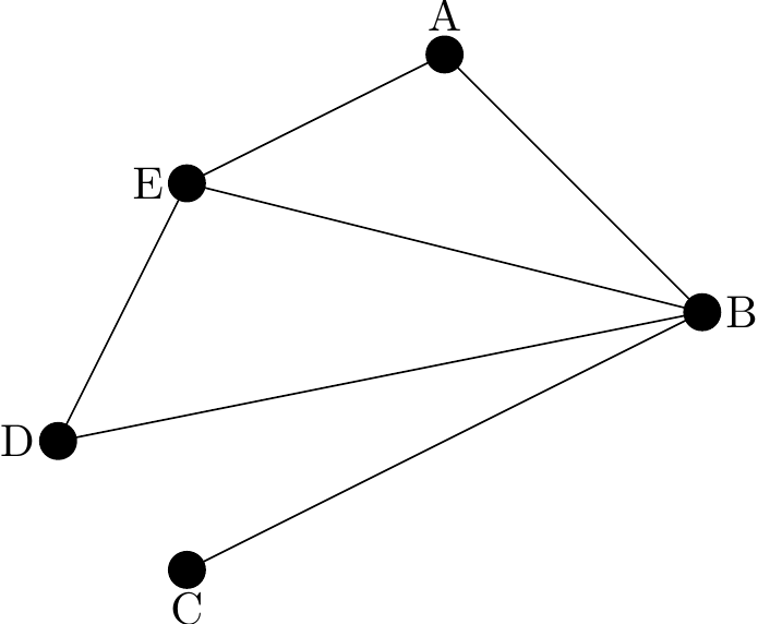
Figure 2.5: A graph to illustrate degree sequence

Note that some texts define the degree sequence of a graph as the degrees of the vertices written in descending order with repetition as necessary. In the above case we would have \(( 4, 3, 2, 2, 1 )\).

2.4 Connected Graphs

We begin with a definition:

A graph is said to be connected if it cannot be expressed as the union of two separated graphs. If a graph is not connected it is said to be disconnected.

This is not a very helpful definition but at least gives the starting idea. We will later also define connected (in a totally equivalent way) as a graph where you can get from any vertex to any other vertex by walking along the edges.

The graph on the left below is connected since it is “in one piece” while the graph on the right is disconnected as it contains two distinct components. See Section 4 for an alternative definition of connected.

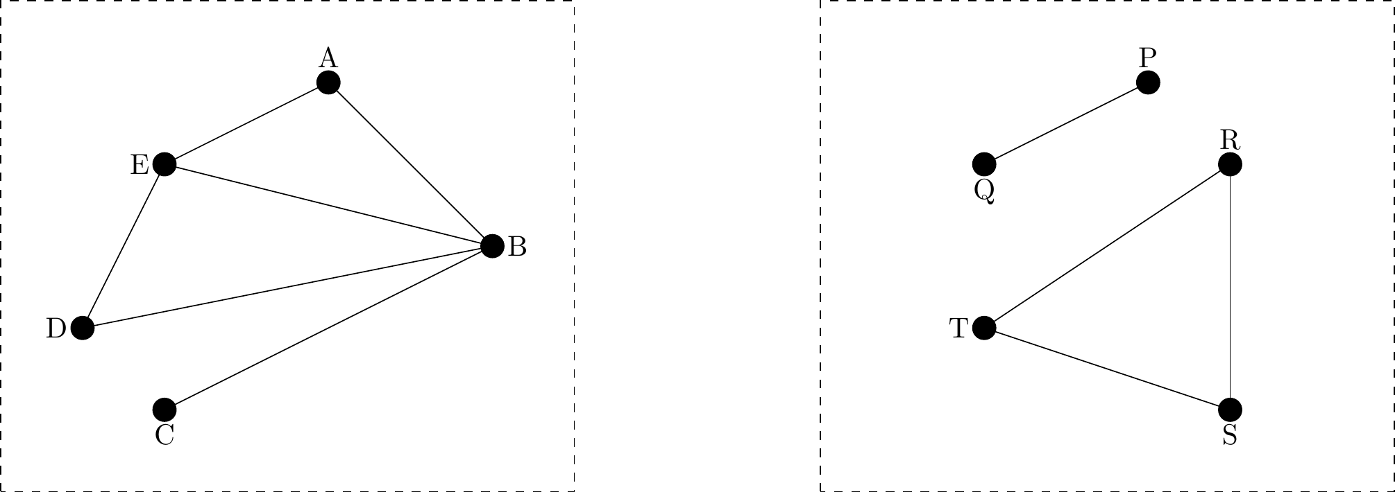
Figure 2.6: Two graphs, each inside a dotted rectangle

When discussing connectedness we sometimes describe a vertex as a cut-vertex or cut-point, to mean that complete removal of that vertex (and all edges incident to it) would leave the remaining graph disconnected.

An edge whose removal would leave to a disconnected graph is known as a cut-edge or bridge.

Example 7 Consider the following graph:

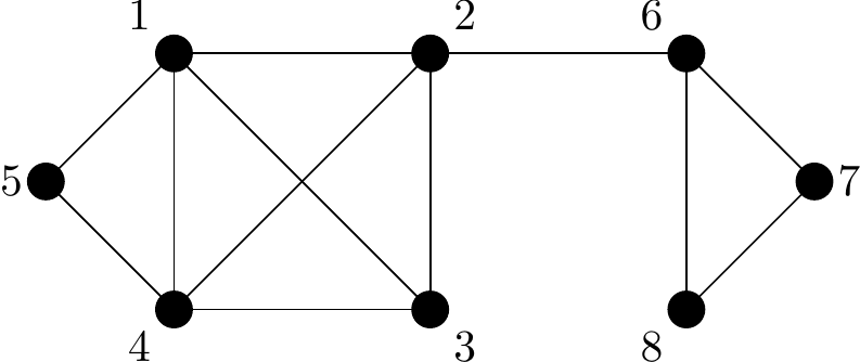
Figure 2.7: A graph to illustrate cut-vertices and cut-edges

Removal of Vertex \(2\) would disconnect the graph, so Vertex \(2\) is known as a cut-vertex. The resulting graph is shown below in Figure 2.8.

Similarly the edge \(\{2,6\}\) is a cut-edge (or bridge) because it’s removal would also disconnect the graph. However, in this case the new disconnected graph would contain more edges than Figure 2.8 because the edges \(\{1,2\}\), \(\{2,3\}\) and \(\{2,4\}\) are not being removed.

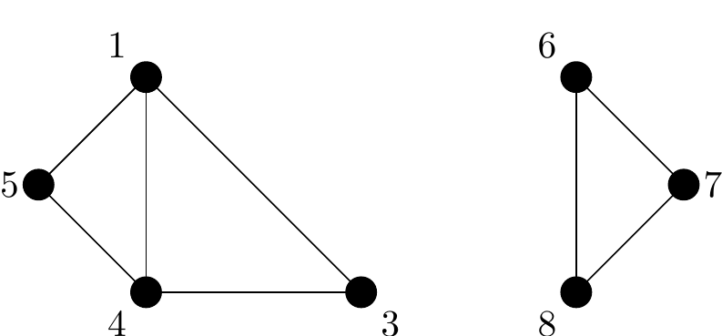
Figure 2.8: Figure 2.7 with Vertex 2 removed

2.5 Common Graphs

In this section we briefly look at different types of common graphs, and common graph properties. Until we reach Section 2.5.6 we shall outlaw the use of parallel edges, so any two vertices are either joined by a single edge, or they are not joined at all.

2.5.1 Regular Graphs

A graph \(G\) is called regular if all vertices of \(G\) have the same degree. A regular graph where all vertices have degree \(k\) is referred to as a \(k\)-regular graph.

We can dive straight into some examples:

Example 8

Figure 2.9: A 0-regular graph

Figure 2.10: A 1-regular graph

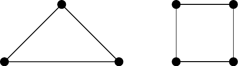
Figure 2.11: Two 2-regular graphs

Practice

Sketch a 2-regular graph on 5 vertices.

1. The Handshaking Lemma tells us that the total degree of any graph is an even number, i.e. twice the number of edges. Hence, it is impossible to construct a \(k\)-regular graph, where \(k\) is odd, on an odd number of vertices.

For example, we cannot have a 3-regular graph on 5 vertices as this would give a degree sum of 15, violating the Handshaking Lemma.

2. A 0-regular graph is called an empty graph.

3. Cycle graphs (see Section 2.5.3) are 2-regular graphs. Also called loops or bands.

4. 3-regular graphs are sometimes called cubic graphs.

Practice

There is only one 3-regular graph on 4 vertices. Can you sketch it?

There are two 3-regular graphs on 6 vertices. Can you sketch them?

There is no 3-regular graphs on 7 vertices. Why?

2.5.2 Complete Graphs

First the definition:

A complete graph, denoted \(K_{n}\), is a graph with \(n\) vertices all of which are adjacent to each other.

Figure 2.12: Complete graphs on 2, 3, 4, 5, 6 and 7 vertices. Courtesy of Wolfram.

The complete graph \(K_{n}\) is regular and each of the \(n\) vertices has degree exactly \(n - 1\). Hence the sum of the degrees is also easy to calculate, it is \(n( n - 1)\), and so by the Handshaking Lemma the number of edges is \(K_{ n}\) is, \(\frac{n( n - 1)}{2}\).

Practice

Check that the two properties stated above hold for the complete graphs shown.

2.5.3 Cycle Graphs

Now for a very popular and useful type of graph for modelling, the cycle graph. But first we shall define the noun cycle in a different way.

A cycle on a graph starts at any vertex, travels through the graph along edges without repeating vertices or edges before ending on the start vertex. In Figure 2.5, BAEB and AEDBA are both cycles while AEDBEA is not a cycle since the vertex E is repeated.

A cycle graph, denoted \(C_n\), is a graph on \(n\) vertices, \(\left\{ v_{0}, v_{1},.\quad.\quad., v_{n-1} \right\}\), with exactly these \(n\) edges \[ \left\{ v_{0}, v_{1} \right\},\left\{ v_{1}, v_{2} \right\},.\quad.\quad.,\left\{ v_{n - 1}, v_{0} \right\}.\]

i.e.\(C_n\) contains a single cycle through all the vertices. The resemblance to a loop or rubber band means these are often called loops or bands.

Example 9

Figure 2.13: \(C_1\)

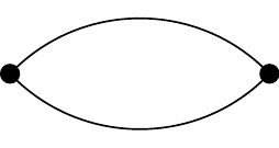
Figure 2.14: \(C_2\)

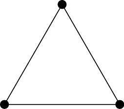
Figure 2.15: \(C_3\)

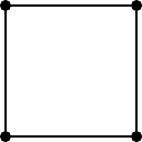
Figure 2.16: \(C_4\)

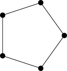
Figure 2.17: \(C_5\)

The first two cycle graphs here are a little silly, and are not often discussed as they contain a self-loop and parallel edges, respectively.

In general a graph that contains no loops or parallel edges is called a simple graph.

You may also note that in every cycle graph, every vertex has degree 2 (as long as we treat \(C_1\) as having degree \(2\) as well).

2.5.4 Bipartite Graphs

Bipartite graphs are much easy to understand from pictures than from the formal definition, but we should at least start with the definition.

A bipartite graph, \(G(V)\) is a graph whose vertices can be partitioned into two disjoint subsets \(V_1\) and \(V_2\), where there are no edges joining vertices that are in the same subset. A vertex in one of the subsets may be joined to all, some, or none of the vertices in the other subset – see the diagrams below.

If the sets \(V_1\) and \(V_2\) are explicitly known we sometimes write \(G(V)=G(V_{ 1}, V_{2}))\).

In the case of a bipartite graph where every vertex of \(V_1\) is joined to every vertex of \(V_2\) then \(G\) is called a complete bipartite graph and is usually denoted \(K_{r,s}\). Where \(r\) and \(s\) are the number of vertices in \(V_1\) and \(V_2\) respectively.

A bipartite graph is usually shown with the two subsets as top and bottom rows of vertices or with the two subsets as left and right columns of vertices like in Figures 2.18 and 2.19.

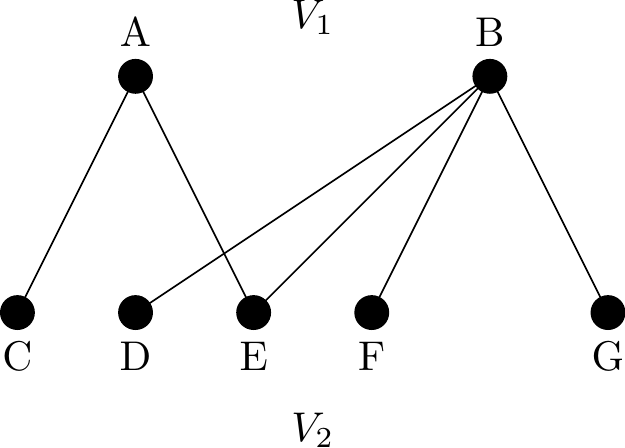
Figure 2.18: A bipartite graph

Figure 2.19: Another bipartite graph

Figure 2.19 is the complete bipartite graph, \(K_{2, 5}\) with \(2+ 5 = 7\) vertices and \(2 \times 5 = \text{10}\) edges. In general, a complete bipartite graph \(K_{ r, s}\) has \(r + s\) vertices and \(r \times s\) edges.

We can think about the topic of regularity in the context of bipartite graphs too. A complete bipartite graph \(K_{ r, s}\) is regular⁸ if and only if \(r = s\). The complete bipartite graph \(K_{ 3, 3}\) shown below is regular as each vertex has degree \(3\).

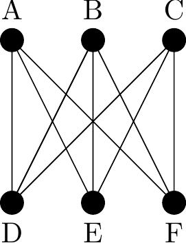
Figure 2.20: The complete bipartite graph \(K_{3,3}\)

A complete bipartite graph of the form \(K_{1, s}\) is called a star graph and \(K_{1, 4}\)is shown below.

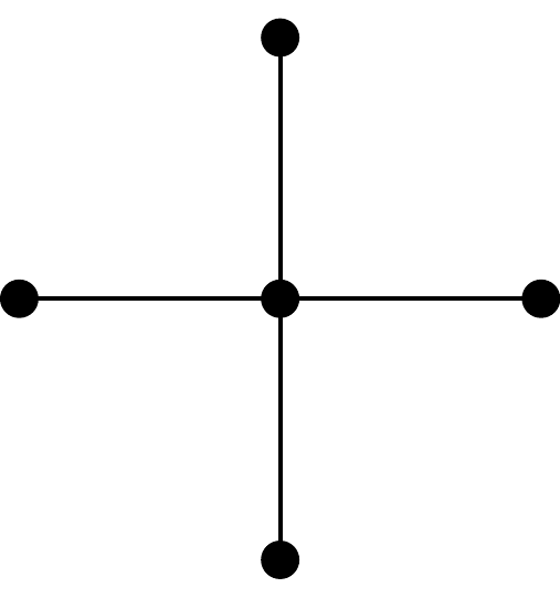
Figure 2.21: The star graph \(K_{1,4}\)

Recall that the locations of the vertices in a diagram of a graph are not fixed. As long as the edges are maintained the vertices can be re-arranged to make the graph easier to understand. To this end identifying that a graph is bipartite can allow a much easier diagram representation, from which the edge connections are simpler to understand. Here is a nice example of the following nice idea.

If all the vertices of a graph can be coloured with two colours in such a way that no two identically coloured vertices are joined by an edge, then the graph is bipartite.

Example 10

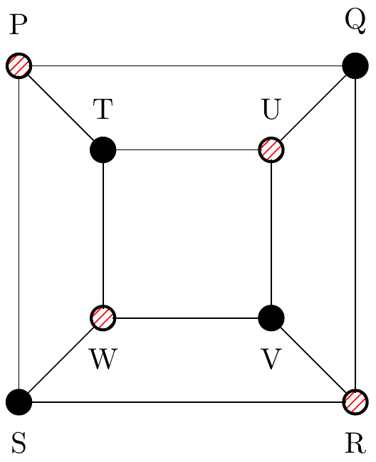
Figure 2.22: A graph on eight vertices, with four highlighted.

The eight vertices in the first image here can be grouped as \(V_1 = \{P,R,U,W \}\) and \(V_2=\{Q,S,T,V\}\) and then re-arranged to form the following image:

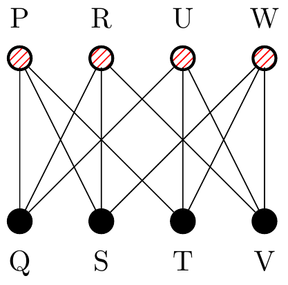
Figure 2.23: The same graph as Figure 2.22 but with vertices moved.

It is now easy to see that the graph is actually just a \(3\)-regular bipartite graph.

Having now seen this idea of moving the vertices around to draw the same graph differently we can introduce a definition we will return to much later, in Section 2.13.

Two graphs with the same number of vertices and edges, with their edges connected in the same way are said to be isomorphic.

It is easy to see that with this definition, that if two graphs have different degree sequences then they must be connected differently, and they are not isopmorphic.

2.5.5 Tree Graphs

A connected graph which contains no cycles in called a tree.

A collection of separate trees (including the case of just one tree!) is called a forest.

This means a forest is actually just any graph with no cycles. Note that a connected graph on \(n\) vertices has fewest edges when it is a tree⁹ (as it has no cycles) and most edges when it is a complete graph. Below is a forest with three components.

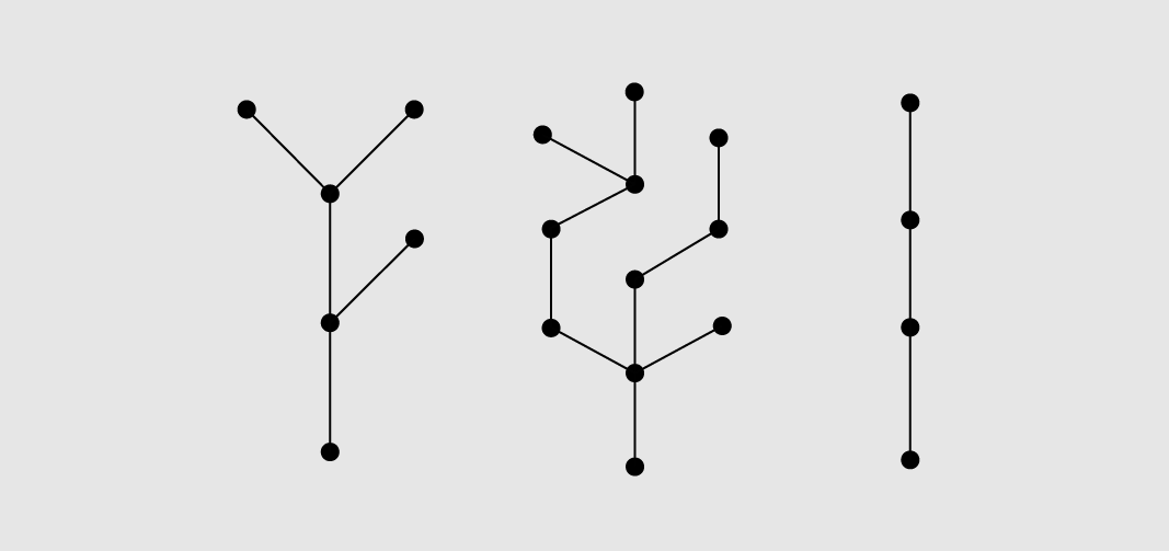
Figure 2.24: Three trees, or one forest.

In Figure 2.24, if one edge were added to connect the first tree to the second tree, and another edge from the second tree to the third tree then one large tree would be formed.

There are in fact a few different, but completely equivalent, ways to define what we mean by a tree. Here is a theorem which summarises the options.

Tree equivalence theorem

Let \(T\) be a graph with \(n > 1\) vertices. The following statements are equivalent:

• \(T\) is a tree.

• \(T\) is cycle-free and has \(n\) – 1 edges.

• \(T\) is connected and has \(n\) – 1 edges.

• \(T\) is connected and contains no cycles.

• \(T\) is connected and each edge is a bridge.

• Any two vertices of \(T\) are connected by exactly one path.

• \(T\) contains no cycles, but the addition of any new edge creates exactly one cycle.

You are free to use any of these definitions when working with trees, as long as you state which one you are using.

Look through the equivalent definitions above and see if you can see why a tree with \(n\) vertices must have \(n-1\) edges under each definition.

2.5.6 Multigraphs

Figure 2.25 shows the graph \(G = \{ V, E \}\) where

\[ V = \{ A, B, C, D \}, \]

and

\[ E = \big\{\{A, B\}, \{B, C\}, \{B, D\}, \{C, D\}, \{C, D\}, \{D, D\}\big\}. \]

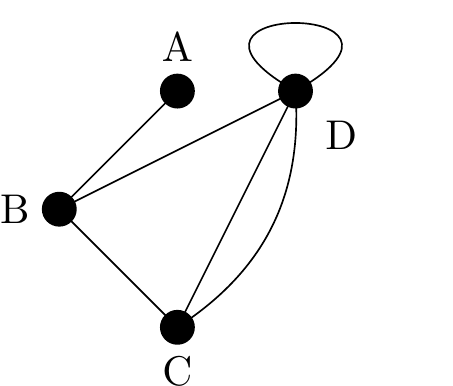
Figure 2.25: An example of a multigraph

A multigraph is a graph that allows the existence of loops and parallel (multiple) edges. Note that not all texts allow multigraphs to have loops and in the case when graphs include loops some authors call them pseudographs.

We shall refer to a graph with parallel edges and/or loops as a multigraph. We study them because when using graphs to model computer networks it is frequently useful to be able to use such loops.

A loop is an edge that links a vertex to itself. In Figure 2.25 the edge {D, D} is a loop and connects vertex D to itself.

If two vertices are joined by more than one edge then these edges are called parallel edges. In Figure 2.25 the two identical edges \(\{C, D\}\) are parallel edges.

Having now defined loops and parallel edges we should make a small note about their implications for certain definitions introduced earlier, in particular how they impact upon the degrees of vertices. We do this to make certain natural results and theorems to apply in all cases.

We define a loop to contribute \(2\) to the degree of the vertex at which it resides, this means the Handshaking Lemma holds for multigraphs.

Similarly parallel edges count separately when calculating vertex degrees, hence vertex \(C\) has a degree of \(3\).

In Figure 2.25, Vertex D therefore has degree 5. The degree sum of the graph is \(1 + 3 + 3 + 5 = 12\) which is twice the number of edges as required by the Handshaking Lemma.

As a final warning some authors use the word multigraph to allow parallel edges but still outlaw loops.

2.6 Walks, Trails & Paths

We begin a new section now, after having discussed a range of standard graphs and their properties we can now discuss things you do with graphs. Once a graph is used to model some real world situation we care about questions to can ask about the graph which may be of real-world use to us. A number of very popular questions about graphs concern how well different vertices are connected to each other, and how easy it is to traverse the entire graph while walking around the edges. To this end we will now introduce three more pieces of terminology.

Warning: When first reading these terms they often sound very similar, but they are in fact describing distinct things.

2.6.1 Walks

A walk of length \(k\) on a graph \(G\) is an alternating sequence of vertices ( \(v_{i}\) ) and edges ( \(e_{i}\) ):

\[ v_{0}, e_{1}, v_{1}, e_{2}, v_{2}, e_{3},\ldots, e_{k}, v_{k} \]

where \(v_{i}\) and \(v_{i + 1}\) are the ends of the edge \(e_{i + 1}\), e.g. \(e_2\) joins \(v_1\) and \(v_2\).

Note that a walk of length \(k\) mentions \(k+1\) vertex names and \(k\) edges.

So the length of a walk is actually the number of edges in the walk not the number of visits to vertices.

For convenience, and ease of reading, we normally omit the edges used on a walk and just list the vertices so that the walk given above is written as \[ v_{0}, v_{1}, v_{2},\ldots, v_{k - 1}, v_{k}.\]

Example 11

A valid walk on the graph in Figure 2.26 is \(1,5,4,3,7,1,6\) and has length \(L=6\).

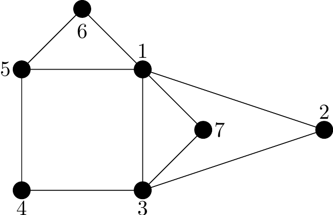
Figure 2.26: A graph to illustrate walks

Note

A walk can repeat vertices and repeat edges. There are no limitations on what a walk can do, beyond being forced to follow edges present.

A walk is said to be closed if its first and last vertices are the same, i.e. \(v_{0} = v_{k}\).

A closed walk, of length \(8\), on Figure 2.26 is given by: \(1, 5, 4, 3, 7, 1, 6, 5, 1\).

2.6.2 Trails

A trail is a walk where all edges used are distinct, but vertices may be repeated.

So the rules to call something a trail are more restrictive than for a walk, and note that a trail is always a walk. It is just one where never uses the same edge twice during the *walk.

An example of a trail on Figure 2.26 would be: \(1, 5, 4, 3, 7, 1, 6, 5\).

In perfect symmetry with our definition from walks, we can also define closed for trails.

A trail is closed if the walk it describes is closed, i.e. it starts and ends at the same vertex.

We invent a new word for a closed trail, we call it a circuit.

So, an example circuit on Figure 2.26 is given by: 1, 2, 3, 1, 5, 4, 3, 7, 1. Note that no edges are repeated but we are allowed to repeat vertices.

2.6.3 Paths

Finally the most restricted walk will be called a path.

A path is a trail where all vertices used are distinct.

Note that distinct vertex visits means that the edges used are bound to be distint too. This means that actually we could alternatively say:

A path is a walk where all edges and all vertices are distinct.

Unsurprisingly we will also use the adjective closed for paths as well, to describe paths which return to their starting vertex.

Note that we need to slightly modify our definition of a path when discussing closed paths. A path is allowed to start and end at the same vertex (this doesn’t count as visiting the vertex twice as we never actually visit it to start with).

An example of a path on Figure 2.26 is given by: \(1, 5, 4, 3, 7\).

A closed path is called a cycle.

A cycle on Figure 2.26 is given by: \(1, 2, 3, 4, 5, 1\). Note that no vertices or edges are repeated.

2.6.4 Interactions

Therefore, all paths are trails and all trails are walks.

We can also use the word open to mean the opposite of closed, i.e. not ending and starting at the same vertex.

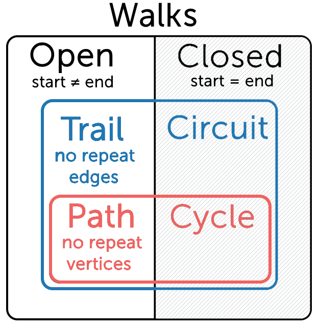
Figure 2.27: An illustration of the overlap between walks, trails, paths, closed and open. Courtesy of mathspace.co

The information given above can be summarised in the following table:

Repeated Vertices allowed?	Repeated Edge(s) allowed?	Open	Closed	Name
Yes	Yes	Yes		Open Walk
Yes	Yes		Yes	Closed Walk
Yes	No	Yes		Trail
Yes	No		Yes	Circuit (Closed Trail)
No	No	Yes		Path
No	No		Yes	Cycle (Closed Path)

Now that we have defined the term path we can provide an alternative definition, to that given Section 2.4, for a graph to be connected.

Alternative definition of connected

A graph is connected if given any two vertices \(v_{i}\) and \(v_{j}\) there is a walk¹⁰ from \(v_{i}\) to \(v_{j}\).

Returning to the example in Section 2.4, reproduced below for completeness, there is clearly a path between all the vertices in the graph on the left and so it is connected. However, in the graph on the right we are unable to, for example, find a path from vertex S to vertex P and so the graph is disconnected.

Figure 2.6: Two graphs, each inside a dotted rectangle

2.7 Eulerian and Hamiltonian Graphs

This section considers special ways of traversing graphs. Examples of graph traversal problems are the Königsberg bridges and Travelling Salesman problems.

2.7.1 Eulerian Graphs

An Euler circuit on a graph, \(G\), is a circuit (closed trail) that uses every edge of \(G\) exactly once. Note that we are allowed to use the same vertex multiple times, but we can only use each edge once.

A graph is Eulerian if it has an Euler circuit.

An Euler trail through a graph, \(G\) is an open trail that passes exactly once through each edge of \(G\).

We say that \(G\) is semi-Eulerian if it has an Euler trail. Note that every Eulerian graph is semi-Eulerian.

It is worth taking a moment to notice the difference between Eulerian and semi-Eulerian, i.e the different between an Euler circuit and an Euler trail. You are recommended to look back at Figure 2.27 to identify what makes a trail also a circuit, i.e. it is closed.

Note the careful wording of the definitions. Since any circuit is always a trail¹¹, saying a graph is Eulerian means it is bound to be also semi-Eulerian.

However, if all trails which visit all the edges must start and end at different vertices then the graph is only semi-Eulerian and not Eulerian. Overall, to say a graph is semi-Eulerian is a less demanding statement than to say it is Eulerian.

Eulerian even-degree graph theorem

Let \(G\) be a connected graph. Then \(G\) is Eulerian if and only if every vertex of \(G\) has even degree.

Corollary to the Eulerian even-degree graph theorem:

A connected graph is semi-Eulerian if and only if there are 0 or 2 vertices of odd degree.

Note that if a semi-Eulerian graph has two vertices of odd degree then any Euler trail must have one of them as its initial vertex and the other as its final vertex. Think about it! One way to try it is to attempt to find an Euler circuit and notice how many visits you need to make to each vertex. Try it out in the examples below.

Example 12

Figure 2.28: A non-Eulerian graph (meaning not Eulerian and not even semi-Eulerian).

Why non-Eulerian?: Four vertices have odd degrees.

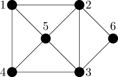
Figure 2.29: A semi-Eulerian graph

Why semi-Eulerian?: Exactly two vertices have odd degree (vertices 1 and 4 both have degree 3). So any Euler trail present must begin at one of these and end at the other. For example, \(12632514534\) but there many others.

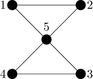
Figure 2.30: An Eulerian graph

Why Eulerian?: The quick answer is that all vertices have even degree (all degree 2). Another way would be to demonstrate an Euler circuit, such as this one: \(1253451\).

The table below provides simple rules that count the number of odd degree vertices in a graph to decide whether or not it has an Euler circuit or Euler trail.

No. of Odd Vertices	For a Connected Graph
0	There is at least one Euler circuit.
1	Not possible
2	No Euler circuit but at least 1 Euler trail.
More than 2	No Euler circuits or Euler trails.

The following algorithm is optional but it provides a relatively simple method for finding an Euler circuit when one exists.

2.7.2 Fleury’s Algorithm

If \(G\) is an Eulerian graph then using the following procedure, known as Fleury’s Algorithm, it is always possible to construct an Euler circuit of \(G\).

Starting at any vertex of \(G\) traverse the edges of \(G\) in an arbitrary manner according to the

following rules:

1. Erase edges as they are traversed and if any isolated vertices appear erase them.
2. At each step use a bridge/cut-edge only if there is no alternative (i.e. don’t cut yourself off from an area by crossing a bridge)

We can now solve the Königsberg bridge problem.

Since every vertex in the Königsberg graph in Figure 2.1 has an odd degree it is not possible to find an Euler circuit of this graph. It is therefore impossible for someone to walk around the city in such a way that each bridge is crossed exactly once and they end up at their starting point.

2.7.3 Hamiltonian Graphs

While the mathematician’s study of graphs concerned their edges, and finding trails through graphs using all the edges. There is a totally analogous question you can ask concerning the vertices. The mathematician William Hamilton studied¹² this problem and his name is given to the property we shall study.

A Hamiltonian cycle on a graph, \(G\), is a cycle (closed path) that uses every vertex of \(G\) exactly once. Note that we do not need to use all the edges. A graph is called Hamiltonian if it has a Hamiltonian cycle.

Note that if your walk around a graph is a path, i.e. it doesn’t repeat any vertices then it couldn’t possible repeat any edges either. Else it would also repeat the vertices at the ends of such edges.

So in the same way that trails were walks that could not repeat edges, and paths were trails that could not repeat vertices¹³, then a Hamiltonian cycle¹⁴ will visit every vertex once but not repeat any edges or vertices

A trail that passes exactly once through each vertex of \(G\) and is not closed is called a Hamiltonian trail.

We say that a graph \(G\) is semi-Hamiltonian if it has at least one Hamiltonian trail.

Note that every Hamiltonian graph is automatically semi-Hamiltonian, this is exactly analogous to the Eulerian / semi-Eulerian relationship from Section 2.7.1.

While we have a theorem that provides necessary and sufficient conditions for a connected graph to be Eulerian (i.e. ‘\(G\) is Eulerian if and only if every vertex of \(G\) has even degree’) there is no such similar characterisation for Hamiltonian graphs – this is one of the unsolved problems in graph theory. In general, it is much harder to find a Hamiltonian cycle than it is to find an Eulerian circuit.

Having said this, for small graphs, using pen and paper it is generally quite simple to identify if a graph is Hamiltonian or not. Indeed if you can find a Hamiltonian cycle then you’ve already proven a graph is Hamiltonian.

Example 13

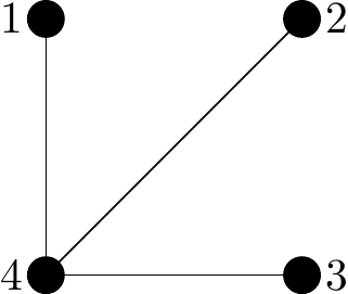
Figure 2.31: A non-Hamiltonian graph (meaning not Hamiltonian and not even semi-Hamiltonian).

Why non-Hamiltonian?: You can quickly check all the possibilities. The issue lies with the fact that upon leaving vertex 4 you are stuck.

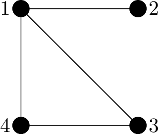
Figure 2.32: A semi-Hamiltonian graph

Why semi-Hamiltonian?: We can easily spot a Hamiltonian trail: for example, 2143 or 2134.

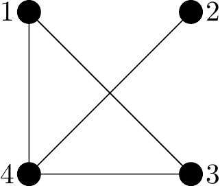
Figure 2.33: A Hamiltonian graph

Why Hamiltonian?: Again there is no known theory, just that if you can find a Hamiltonian cycle then is is Hamiltonian.

Here we can find 12341 fairly easily. Notice that this Hamiltonian cycle doesn’t use all the edges (indeed it cannot else it would repeat vertices).

The famous Travelling Salesperson Problem (TSP) searches for the most efficient (least total distance) Hamiltonian cycle. That is, a route that visits every city on some map (each exactly once) with minimal total distance travelled. This obviously has real-world applications. However, since finding Hamiltonian cycles is a very difficult problem for large graphs it is not all that surprising that this remains an unsolved problem.

Here’s a potential useful memory aid for this chapter:

An Eulerian circuit traverses every Edge in a graph exactly once, and may repeat vertices.

A Hamiltonian cycle, on the other hand, visits each Vertex in a graph exactly once but does not need to use every edge.

The fact that Euler and Edge begin with the same letter can be useful for remembering. Both Hamilton and Euler studied the principle of ‘visiting the entire graph’ just meant to visit every vertex and the other to visit every edge.

2.8 Digraphs (Directed Graphs)

The graphs that we have been studying up to now have all been undirected graphs in the sense that the edges have no orientation/direction/arrows. In this section we extend the notion of a graph to include graphs in which “edges have a direction”. These kind of graphs are known as directed graphs, or digraphs for short.

As shown in the diagram below the direction of an edge is signified by a small arrow drawn on the edge and the purpose is to state that movement between two vertices is only possible in the specified direction. The terminology for digraphs is essentially the same as for undirected graphs except that it is commonplace to use the term arc instead of edge.

Digraphs can be used to model real-life situations such as flow in pipes, traffic on roads, route maps for airlines and hyperlinks connecting web-pages. For example, a hyperlink is a one-directional edge (an arc) which takes you from one site to another, unless you add a link on the resulting page back to the previous page then you cannot get back (without using separate in-built browser functions).

Example 14

Figure 2.34 below shows a digraph on four vertices with six arcs.

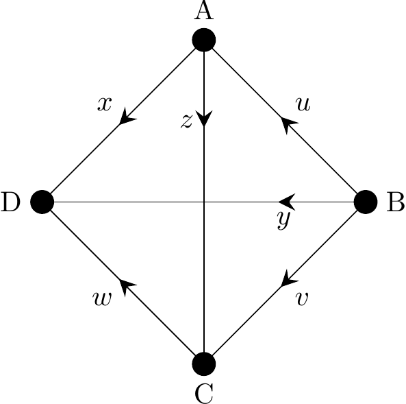
Figure 2.34: A directed graph (or digraph)

Considering the arc labelled \(x\), we say that \(x\) goes from A to D with A being the initial vertex and D the terminal vertex of \(x\).

Note that with digraphs it is now very important when describing an edge, which vertex you mention first, the order now matters. So when listing edges of digraphs we generally use the \((A,B)\) bracket notation, rather than \(\{A,B\}\) since we use \((\) and \()\) normally in maths when the order of elements matter.

2.8.1 In-degree and Out-degree

Previously the degree of a vertex was just the number of edge ends incident at that vertex. Now it makes sense to count in-coming directed edges and out-going directed edges separately. Hence the following definitions.

The in-degree of a vertex is the number of arcs that terminate at that vertex.

For example, the in-degree of vertex C in Figure 2.34 is \(2\).

The out-degree of a vertex is the number of arcs that originate at that vertex.

For example, the out-degree of vertex B in Figure 2.34 is \(3\).

2.8.1.1 The Handshaking (Di)Lemma

The Handshaking Lemma has a much simpler to understand version for digraphs:

The Handshaking Lemma for Digraphs

In any digraph the sum of the out-degrees, equals the sum of the in-degrees, equals the number of arcs.

This is very obvious once you notes that every arc contributes exactly once to the out-degree total and exactly once to the in-degree total (because it has two ends!).

We can also define equivalent versions of the degree sequence for digraphs.

The in-degree sequence of a digraph is a bracketed list of the in-degrees of all the vertices in ascending order with repetition as necessary.

The out-degree sequence of a digraph is a bracketed list of the out-degrees of all the vertices in ascending order with repetition as necessary.

Example 15

Consider the following digraph.

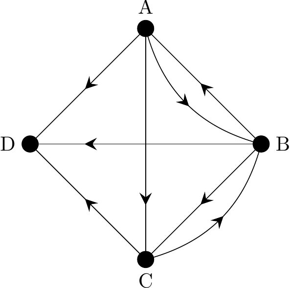
Figure 2.35: A directed graph (or digraph)

1. Determine the in-degree and out-degree of the vertices and show that the Handshaking (Di)Lemma holds
2. Write down the in-degree and out-degree sequences.

Answers:

1. We create this table of in-degrees and out-degrees:

Degree type	A	B	C	D	Total
Out-degree	3	3	2	0	8
In-degree	1	2	2	3	8

The sum of the out-degrees (8) equals the sum of the in-degrees (8) and these values both equal the number of edges (8).

The Handshaking (Di)Lemma therefore holds.

2. From the table in part (1), the in-degree sequence is \((1, 2, 2, 3)\) and the out-degree sequence is \((0, 2, 3, 3)\).

2.9 Underlying Graph

The underlying graph of a digraph is the undirected graph obtained when the arrows are removed from the digraph (but the edges are kept), i.e. when you choose to ignore the directions mandated by the arrows.

Example 16

The graph underlying the digraph in Figure 2.34 is the undirected graph shown below.

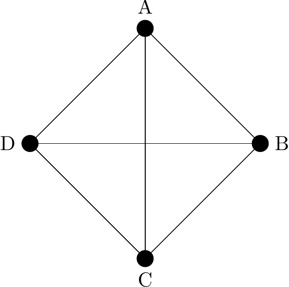
Figure 2.36: The underlying (undirected) graph derived from Figure 2.34.

Note that we have basically just removed the arrows, so what we may have been calling directed arcs we now just call edges again.

Earlier we discussed the idea of a connected graph, in Section 2.4. This concept could become complicated for digraphs if we choose to study them. However, a perfectly useful definition that works well for working with digraphs is actually very straightforward, and reduces the problem to the one we have already studied.

Definition of connected for digraphs

We will say a digraph is connected if the underlying graph (i.e. the one with the arrows removed) is connected (using our earlier definition for connected from undirected graphs).

Note this will contrast with the following section, Section 2.9.1, where we discuss walks, trails and paths for digraphs where we will demand that the directions given by the arrows are always respected.

2.9.1 Walks, Trails and Paths on Digraphs

The concept of walks, trails and paths carries over from undirected graphs to digraphs in a very simple fashion. We just must remember that on a digraph we can only move along an edge in a single direction, i.e. the direction in which the arrow is pointing.

Arrows must be obeyed!

Find a walk, trail and path on the digraph shown below.

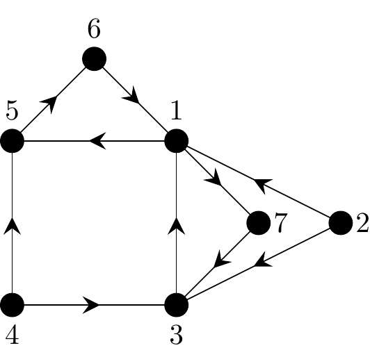
Figure 2.37: A sample digraph to illustrate walks, trails and paths

Reminder of definitions

A walk has no restrictions other than following directed edges. It can repeat edges and vertices if it wishes.

A trail is a walk which cannot repeat any edge used.

A path is a trail (or walk) which cannot repeat any vertex visit (except for starting and ending at the same vertex, which is allowed and would make it closed).

Sample solutions to exercise in Figure 2.37:

• One example of a walk is given by: 1, 5, 6, 1, 7, 3, 1, 5, 6.
• One example of a trail is given by: 1, 5, 6, 1, 7, 3.
• One example of a path is given by: 1, 5, 6.

All other terminology carries across too, so we can discuss open or closed walks, paths and trails. We will return to discuss the adjectives Eulerian and Hamiltonian for directed graphs in Sections 2.10.3 and 2.10.4, but first we shall make a practical diversion.

2.10 Adjacency Matrices

We now move onto a more practically useful topic for the applications of matrices in computing and many other areas. Most work with networks and graphs nowadays involves the use of computers. Up to now we have only considered graphs where the number of edges and vertices is relatively small so that they can be easily be shown in diagram form. However, as graphs become large it is no longer feasible to display them visually. When storing a graph on a computer it is useful to represent it in matrix form. It turns out that there are nice algorithms for calculating paths, trails and circuits, for example, using matrices and just standard matrix multiplication methods. This

2.10.1 Adjacency Matrix of an Undirected Graph

In Section 2.2.1 we defined an undirected graph to be a graph in which the edges have no arrows. Hence, all edges are bidirectional. For example, in the graph shown in Figure 2.36 the edge \(\left\{ A, B \right\}\) is considered identical to the edge \(\left\{ B, A \right\}\).

Given the way we will define adjacency matrices we will provide definitions for undirected and directed graphs separately, but you will see they are really the same if you consider bidirectional edges at providing one edge in each direction.

If \(G\) is a graph with \(n\) vertices, its adjacency matrix, normally called \(A\), is defined as an \(n \times n\) matrix whose ij-th entry is the number of edges joining vertex \(i\) and vertex \(j\).

Recall that when working with matrices the rule is always Rows fiRst, Columns seCond. So in the definition above a single edge joining vertex \(7\) to vertex \(3\), in a graph with \(10\) vertices, means a \(1\) is placed in Row 7, Column 2 of the adjacency matrix. Let’s see a full example.

Example 17

Determine an adjacency matrix for following graph.

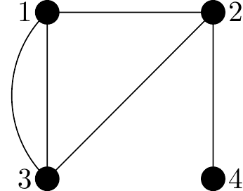
Figure 2.38: A graph used to illustrate an adjacency matrix

Solution:

This graph has \(4\) vertices and so the adjacency matrix will have dimension, \(4 \times 4\). It’s standard practice to include the names of the vertices along the left and top of the matrix so that we know which rows correspond with which vertices. Here’s our template we need to fill:

\[ \begin{matrix} & \begin{matrix}1&2&3&4\end{matrix} \\ \begin{matrix}1\\2\\3\\4\end{matrix} \hspace{-1em} & \begin{pmatrix} \cdot&\cdot&\cdot&\cdot \\ \cdot&\cdot&\cdot&\cdot \\\cdot&\cdot&\cdot&\cdot \\\cdot&\cdot&\cdot&\cdot \end{pmatrix} \end{matrix} \]

We can start with row 1. This contains information about edges that leave vertex 1 and join to other vertices.

• No edges connect vertex 1 to vertex 1, so the entry in Row1/Column1 is a \(0\).
• \(1\) edge connects vertex 1 to vertex 2, so the entry in Row1/Column2 is a \(1\).
• \(2\) edges connect vertex 1 to vertex 3, so the entry in Row1/Column3 is a \(2\).
• No edges connect vertex 1 to vertex 4, so the entry in Row1/Column4 is a \(0\).

Here is row 1 completed:

\[ \begin{matrix} & \begin{matrix}1&2&3&4\end{matrix} \\ \begin{matrix}1\\2\\3\\4\end{matrix} \hspace{-1em} & \begin{pmatrix} 0&1&2&0 \\ \cdot&\cdot&\cdot&\cdot \\\cdot&\cdot&\cdot&\cdot \\\cdot&\cdot&\cdot&\cdot \end{pmatrix} \end{matrix} \]

Next for row 2. We look at what edges leave vertex 2 and join to other vertices.

• \(1\) edge connects vertex 2 to vertex 1, so the entry in Row2/Column1 is a \(1\).
• No edges connect vertex 2 to vertex 2, so the entry in Row2/Column2 is a \(0\).
• \(1\) edge connects vertex 2 to vertex 3, so the entry in Row2/Column3 is a \(1\).
• \(1\) edge connects vertex 2 to vertex 4, so the entry in Row2/Column4 is a \(1\).

So, here are the first two rows completed:

\[ \begin{matrix} & \begin{matrix}1&2&3&4\end{matrix} \\ \begin{matrix}1\\2\\3\\4\end{matrix} \hspace{-1em} & \begin{pmatrix} 0&1&2&0 \\ 1&0&1&1 \\\cdot&\cdot&\cdot&\cdot \\\cdot&\cdot&\cdot&\cdot \end{pmatrix} \end{matrix} \]

You should complete the final two rows yourself, and reach the following matrix:

\[ \begin{matrix} & \begin{matrix}1&2&3&4\end{matrix} \\ \begin{matrix}1\\2\\3\\4\end{matrix} \hspace{-1em} & \begin{pmatrix} 0&1&2&0 \\ 1&0&1&1 \\ 2&1&0&0 \\ 0&1&0&0 \end{pmatrix} \end{matrix} \]

This is the adjacency matrix for the graph in Figure 2.38.

There are a number of points worth noting arising from this example, and other similar ones.

• A graph can be represented by several adjacency matrices as different labelling of the vertices produces different matrices. In our case we used the natural row and column labelling \(1,2,3,4\). While you should always use the same order for columns and rows, if the vertices have other names you might choose any order. For example, if vertices are called Frog (F), Cat (C) and Rabbit (R) there may be no natural order and various template options exist, such as:

\[ \begin{matrix} & \begin{matrix}F&C&R\end{matrix} \\ \begin{matrix}F\\C\\R\end{matrix} \hspace{-1em} & \begin{pmatrix} ~\cdot~&~\cdot~&~\cdot~ \\ ~\cdot~&~\cdot~&~\cdot~ \\~\cdot~&~\cdot~&~\cdot~ \end{pmatrix} \end{matrix} \qquad \textrm{ and } \qquad \begin{matrix} & \begin{matrix}C&R&F\end{matrix} \\ \begin{matrix}C\\R\\F\end{matrix} \hspace{-1em} & \begin{pmatrix} ~\cdot~&~\cdot~&~\cdot~ \\ ~\cdot~&~\cdot~&~\cdot~ \\~\cdot~&~\cdot~&~\cdot~ \end{pmatrix} \end{matrix} \]

• In the matrix \(A\), the entry \(a_{ ij}\) records the number of edges joining vertices \(i\) and \(j\). So for most standard graphs you will study, every entry will be either a \(0\) or a \(1\) since it is only multigraphs and graphs with loops where you can get values above \(1\). The example in Figure 2.38 is unusual in this regard, in that it contains parallel edges.

• For an undirected simple¹⁵ graph:

Sum of Row \(j\) = Sum of Column \(j\) = Degree of vertex \(j\) .

• The adjacency matrix for an undirected graph is always going to be symmetric, i.e. \(A = A^{ T}\).

• The entries on the main diagonal are all 0 unless the graph has any loops.

Now that we have a definition of an adjacency matrix, and know how to construct one from a picture of a graph. There is another skill which we can develop, namely to construct a picture of a graph given its adjacency matrix.

When doing this you may not always place your vertices in the most ideal positions when you begin your sketch. Placing them non-ideally could result in lots of criss-crossing edges in your final picture, so feel free to have a glance at the full matrix first to try and avoid this and draw your vertices as nicely spread as possible, then you hopefully won’t need to redraw your graph later to make it look more aesthetically pleasing.

Example 18

Given the adjacency matrix below, construct the associated (multigraph), \(G\).

\[ \begin{matrix} & \begin{matrix}1&2&3&4\end{matrix} \\ \begin{matrix}1\\2\\3\\4\end{matrix} \hspace{-1em} & \begin{pmatrix} 0&2&0&1 \\ 2&2&1&1 \\ 0&1&0&1 \\ 1&1&1&0 \end{pmatrix} \end{matrix} \]

Solution:

The matrix has dimension \(4 \times 4\) and so the graph has \(4\) vertices. Their names have already been provided too, via the row and column labels.

Note that a loop is defined to contribute 2 to the degree of a vertex. So the \(2\) in second row, second column, is fulfilled by drawing a single edge joining vertex \(2\) to itself. This is a conventional definition that we discussed earlier in Multigraphs Section 2.5.6 to keep the Handshaking Lemma working.

We begin by loosely drawing four vertices, we go with a square arrangement for lack of any other knowledge.

We proceed as follows processing one row of the matrix \(A\) at a time:

• Entry in Row1/Column1 is a ‘0’ so 0 edges connect vertex 1 to vertex 1.
• Entry in Row1/Column2 is a ‘2’ so 2 edges connect vertex 1 to vertex 2.
• Entry in Row1/Column3 is a ‘0’ so 0 edges connect vertex 1 to vertex 3.
• Entry in Row1/Column4 is a ‘1’ so 1 edge connects vertex 1 to vertex 4.

So temporarily we have drawn this graph:

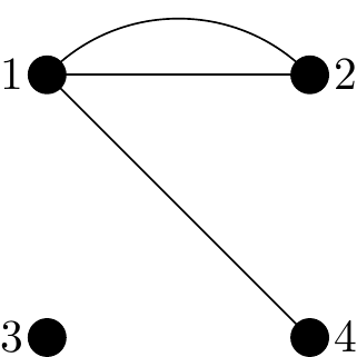
Figure 2.39: Our graph \(G\) having drawn only the edge from vertex 1 so far.

Next for row 2 (i.e. edges that leave vertex 2):

• Entry in Row2/Column1 is a ‘2’ so 2 edges connect vertex 2 to vertex 1.
• Entry in Row2/Column2 is a ‘2’ so vertex 2 has a self-loop.
• Entry in Row2/Column3 is a ‘1’ so 1 edge connects vertex 2 to vertex 3.
• Entry in Row2/Column4 is a ‘1’ so 1 edge connects vertex 2 to vertex 4.

We don’t need to draw edges which have already been drawn.

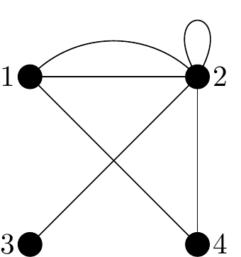
Figure 2.40: Our graph \(G\) having drawn only the edges from vertices 1 and 2 so far.

Now for rows 3 and 4 of the adjacency matrix:

• Entry in Row3/Column1 is a ‘0’ so 0 edges connect vertex 3 to vertex 1.
• Entry in Row3/Column2 is a ‘1’ so 1 edge connects vertex 3 to vertex 2.
• Entry in Row3/Column3 is a ‘0’ so 0 edges connect vertex 3 to vertex 3.
• Entry in Row3/Column4 is a ‘1’ so 1 edge connects vertex 3 to vertex 4.
• Entry in Row4/Column1 is a ‘1’ so 1 edge connects vertex 4 to vertex 1.
• Entry in Row4/Column2 is a ‘1’ so 1 edge connects vertex 4 to vertex 2.
• Entry in Row4/Column3 is a ‘1’ so 1 edge connects vertex 4 to vertex 3.
• Entry in Row4/Column4 is a ‘0’ so 0 edges connect vertex 4 to vertex 4.

The graph corresponding to the adjacency matrix is therefore:

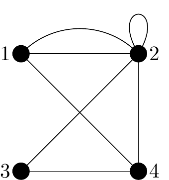
Figure 2.41: Our graph \(G\) having drawn all the edges.

Here is a more ‘standard’ example. A graph with no parallel edges or loops, i.e. a simple graph.

Example 19

Here is the adjacency matrix of a graph on \(5\) vertices:

\[ \begin{matrix} & \begin{matrix}1&2&3&4&5\end{matrix} \\ \begin{matrix}1\\2\\3\\4\\5\end{matrix} \hspace{-1em} & \begin{pmatrix} 0&1&0&0&1 \\ 1&0&0&0&1 \\ 0&0&0&1&0 \\ 0&0&1&0&1 \\ 1&1&0&1&0 \end{pmatrix} \end{matrix} \]

Here is one sketch of it.

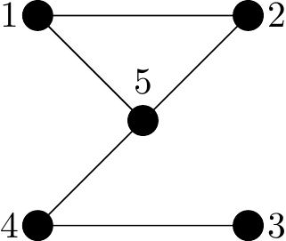
Figure 2.42: A sketch of the graph with adjacency matrix above.

Look through the edges present, and not present in the graph and check you can see how they correspond with the entries of the adjacency matrix.

There are three things worthy of note about the adjacency matrix of all simple graphs like that in Figure 2.42:

• every entry of the matrix is either a \(0\) or a \(1\),
• the adjacency matrix is symmetric,
• the matrix diagonal from top left to bottom right (the leading diagonal) is all zeroes.

You should think about all three and convince yourself they will always be true for such graphs.

2.10.2 Adjacency Matrix of a directed graph

We have formally only looked at adjacency matrices of undirected graphs so far, i.e. where edges have no arrows. The definition for directed graphs is essentially the same, but each directed edge only contributes a single \(1\) to the adjacency matrix now.

For undirected graphs the edge from vertex \(4\) to vertex \(2\) appeared in the adjacency matrix as both a \(1\) in Row 4, Column 2 and also in Row 2, Column 4.

For a directed graph a directed edge from vertex \(4\) to vertex \(2\) only contributes to Row 4, Column 2, since it is an edge from \(4\) to \(2\) and not an edge from \(2\) to \(4\).

So for simple graphs (no parallel edges, and no loops):

The adjacency matrix of a digraph having \(n\) vertices is a \(n \times n\) matrix.

For each directed edge from a vertex \(v_i\)¹⁶ to a vertex \(v_j\)¹⁷ we place a \(1\) in the i-th row and j-th column. Otherwise we place a \(0\) in that position.

i.e.

\[ \text{Entry \((i,j)\) in the matrix} = \begin{cases} 0 & \text{if arrow from \(i\) to \(j\)} \\ 1 & \text{if NO arrow from \(i\) to \(j\)} \end{cases} \]

We used generic names \(v_i\) and \(v_j\) here in case the vertices are not numbered \(1,2,3,\ldots\).

In the case that our directed graph has loops or parallel edges, each separated directed edge contributes \(+1\) to its corresponding matrix entry. Thus four arcs from vertex \(3\) to vertex \(2\) will create an entry in the matrix of value \(4\) in row 3, column 2. So entries could be larger than \(1\).

Example 20

Determine an adjacency matrix for the digraph shown below,

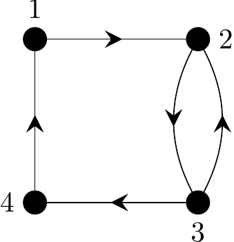
Figure 2.43: A directed graph to illustrate adjacency matrices

Solution:

• The digraph has \(4\) vertices and so the adjacency matrix will have dimension \(4 \times 4\);
• There is an arc from vertex 1 to vertex 2, so the entry in Row1/Column2 is a \(1\);
• There is an arc from vertex 2 to vertex 3, so the entry in Row2/Column3 is a \(1\);
• There is an arc from vertex 3 to vertex 2, so the entry in Row3/Column2 is a \(1\);
• There is an arc from vertex 3 to vertex 4, so the entry in Row3/Column4 is a \(1\);
• There is an arc from vertex 4 to vertex 1, so the entry in Row4/Column1 is a \(1\);
• All other entries in the adjacency matrix will be zero

From the calculations above an adjacency matrix for the digraph is therefore:

\[ \begin{matrix} & \begin{matrix}1&2&3&4\end{matrix} \\ \begin{matrix}1\\2\\3\\4\end{matrix} \hspace{-1em} & \begin{pmatrix} 0&1&0&0 \\ 0&0&1&0 \\ 0&1&0&1 \\ 1&0&0&0 \end{pmatrix} \end{matrix} \]

• The total number of 1’s in an adjacency matrix equals the number of arcs in the digraph.
• In general, the adjacency matrix is not symmetric for a digraph;
• The number of 1’s in row \(i\) of an adjacency matrix corresponds to the out-degree of this i-th vertex;
• The number of 1’s in column \(j\) of an adjacency matrix corresponds to the in-degree of this j-th vertex.

2.10.3 Eulerian Digraphs

Recalling now our definition of Eulerian, for a digraph this will mean finding a path which follows the arrows and visits every edge of the graph exactly once.

Definition of an Eulerian digraph

A digraph \(G\) is Eulerian if it is connected and there exists a closed trail (circuit) which uses each arc exactly once.

Vertices however, can be repeated. This definition is essentially the same as for undirected graphs, see Section 2.7.1, except that we can only traverse the graph in the direction of the arrows.

We have a similar theorem which allows us to quickly identify if a digraph is Eulerian or not.

Eulerian in-out degree theorem

Let \(G\) be a connected digraph. Then \(G\) is Eulerian if and only if the in-degree of each vertex equals its out-degree.

It is worth comparing this with the Eulerian even-degree graph theorem from 2.7.1.

We shall illustrate the concepts with an extended example.

Example 21

Consider the following digraph, \(D\).

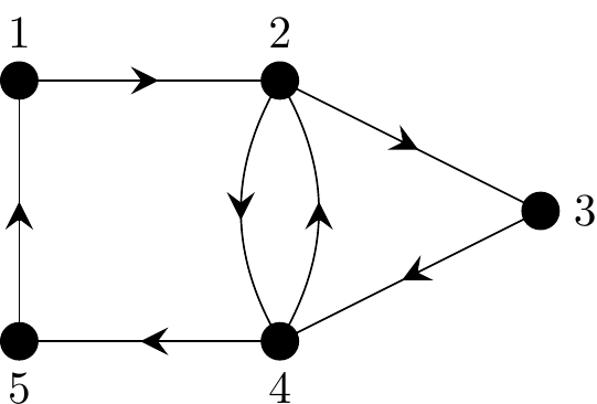
Figure 2.44: A directed graph to illustrate Eulerian paths

1. Determine an adjacency matrix for \(D\).
2. Is \(D\) Eulerian? Either state an Euler circuit or explain why \(D\) is not Eulerian.

Solution:

1. The digraph has 5 vertices and so the adjacency matrix will have dimension \(5 \times 5\).

The adjacency matrix is as follows:

\[ A = \begin{matrix} & \begin{matrix}1&2&3&4&5\end{matrix} \\ \begin{matrix}1\\2\\3\\4\\5\end{matrix} \hspace{-1em} & \begin{pmatrix} 0&1&0&0&0 \\ 0&0&1&1&0 \\ 0&0&0&1&0 \\ 0&1&0&0&1 \\ 1&0&0&0&0 \end{pmatrix} \end{matrix} \]

Here are the full gory details:

• There is an arc from vertex 1 to vertex 2, so the entry in Row1/Column2 is a \(1\);

• There is an arc from vertex 2 to vertex 3, so the entry in Row2/Column3 is a \(1\);

• There is an arc from vertex 2 to vertex 4, , so the entry in Row2/Column4 is a \(1\);

• There is an arc from vertex 3 to vertex 4, , so the entry in Row3/Column4 is a \(1\);

• There is an arc from vertex 4 to vertex 2, , so the entry in Row4/Column2 is a \(1\);

• There is an arc from vertex 4 to vertex 5, so the entry in Row4/Column5 is a \(1\);

• There is an arc from vertex 5 to vertex 1, so the entry in Row5/Column1 is a \(1\);

• All other entries in the adjacency matrix will be zero.

2. Recall that the row sums of \(A\) give the out-degrees while the column sums provide the in-degrees of the vertices. We construct the following table:

Vertex	Out-degree	In-degree
1	1	1
2	2	2
3	1	1
4	2	2
5	1	1

This digraph is Eulerian as the out-degree of each vertex is the same as its in-degree. i.e. Colloquially every vertex has the same number of arrows coming in as going out.

Can we find an Euler circuit? Just try!

An example Euler circuit is given by: \(1, 2, 3, 4, 2, 4, 5, 1\).

The same definition for semi-Eulerian carries over from previously. It is left as an exercise for the reader to see why what the requirement is for a digraph to be semi-Eulerian (but not Eulerian). Here is the answer to think about:

• For all expect two vertices the in-degree and out-degree must match exactly;
• One of these two vertices has an in-degree exactly \(1\) higher than its out-degree;
• The other of these two vertices has an out-degree exactly \(1\) higher than its its-degree;

2.10.4 Hamiltonian Digraphs

Now for the Hamiltonian version on directed graphs. Recall we will be looking for a path which follows the arrows but this time visits every vertex of the graph exactly once. This will necessarily force us to never use any edge more than once. Note, however, that we don’t need to use all edges.

A digraph \(G\) is Hamiltonian if it is connected and there exists a closed cycle which visits every vertex exactly once.

This definition is essentially the same as the for undirected graphs, see Section 2.7.3, except that we can only traverse the graph in the direction of the arrows.

Just as for Hamiltonian graphs with undirected edges there is no known result to determine if a graph is actually Hamiltonian beyond finding such a cycle.

Example 22

Consider the same graph as in Figure 2.44 which we repeat here for convenience:

Figure 2.44: A directed graph to illustrate Eulerian paths

A Hamiltonian cycle for this digraph can be found to be \(1, 2, 3, 4, 5, 1\).

We have been able to visit each vertex exactly once and return to our starting vertex.

2.11 Adjacency Matrices & Paths

Now we will see the power of using matrices to represent graphs. Adjacency matrices can be used to determine the number of paths of different lengths between vertices without having to manually and systematically count them all.

We first nite that in an adjacency matrix the entry at position \((i, j)\) corresponds to the number of paths of length 1 between vertex \(v_{ i}\) and vertex \(v_{ j}\). Note the weird choice of phrase here, path of length 1 just means a single arc, but can be made more general to longer lengths in a moment.

It is also possible to construct matrices that provide information on paths of length other than 1 between vertices.

First a little motivation, note that if we want to count all the paths of length \(2\) from vertex A to vertex B in a graph, we need to:

• consider all possible edges out of vertex A;
• see where each such edges goes;
• see whether for each such destination, there is an edge immediately to vertex B;
• add together all the examples found.

Imagine instead we have the adjacency matrix of this graph, where rows \(1\) and \(2\) corresponds to vertices A and B respectively. To find paths of length \(2\) we can do the following:

• look at row \(1\)¹⁸ of the matrix for places where it is not zero;
• for each entry above that is not zero, identify which column it is in;
• for each such column, look at the matching row number and see if there is an edge straight to vertex B (i.e. in column \(2\));
• add up all the examples found.

We shall not go into the details here, but this latter process is actually just equivalent to multiplying the matrix \(A\) by itself and looking for the entry in row 1 column 2!

Theorem for counting paths

The matrix \(A^2 = A \times A\) contains in its entries the number of paths of length exactly 2 from each vertex to each other vertex.

And in general, if we calculate the \(k\)-th power of the adjacency matrix \(A\) then the entry at position \((i,j)\) of the matrix \(A^{ k}\) indicates the number of paths of length \(k\) between vertex \(v_{i}\)and vertex \(v_{j}\).

This is a pretty amazing fact, and it is just a result of our clever definition for matrix multiplication.

Example 23

Let \(D\) be a digraph with 5 vertices as shown:

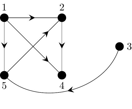
Figure 2.45: A directed graph to illustrate path counting

An adjacency matrix is given by

\[ A = \begin{matrix} & \begin{matrix}1&2&3&4&5\end{matrix} \\ \begin{matrix}1\\2\\3\\4\\5\end{matrix} \hspace{-1em} & \begin{pmatrix} 0&1&0&1&1 \\ 0&0&0&1&0 \\ 0&0&0&0&1 \\ 0&0&0&0&0 \\ 0&1&0&0&0 \end{pmatrix} \end{matrix} \]

If a path of length 1 exists between two vertices (i.e. vertices are adjacent) then there is a 1 in the corresponding position in the adjacency matrix, \(A\). Here, for example, inspection of \(A\) reveals the following paths of length 1:

• from vertex 1 to vertices 2, 4 and 5
• from vertex 2 to vertex 4
• from vertex 3 to vertex 5
• from vertex 5 to vertex 2.

There are no paths of length 1 from vertex 4 to any of the other vertices.

But if we want a path of length \(2\) from, say, vertex 1 to vertex 2, we are looking for a 1 in the first row¹⁹ and a 1 in the correspnding position of the second column²⁰.

Here is the calculation:

\[ A^2 = \begin{pmatrix} \color{crimson}0&\color{crimson}1&\color{crimson}0&\color{crimson}1&\color{crimson}1 \\ 0&0&0&1&0 \\ 0&0&0&0&1 \\ 0&0&0&0&0 \\ 0&1&0&0&0 \end{pmatrix} \begin{pmatrix} 0&\color{crimson}1&0&1&1 \\ 0&\color{crimson}0&0&1&0 \\ 0&\color{crimson}0&0&0&1 \\ 0&\color{crimson}0&0&0&0 \\ 0&\color{crimson}1&0&0&0 \end{pmatrix} = \begin{pmatrix} 0&\color{crimson}1&0&1&0 \\ 0&0&0&0&0 \\ 0&1&0&0&0 \\ 0&0&0&0&0 \\ 0&0&0&1&0 \end{pmatrix} \]

The scalar product of row 1 with column 2 results in the entry present in row 1 columns 2 of the answer. This value, in entry \((1,2)\) of \(A^2\) tell us how many paths there are of length \(2\) from vertex 1 to vertex 2. In this case there is only 1 path.

What is this path? If we look carefully at the calculation of the \((1,2)\) entry of \(A^2\) we see the value \(1\) appeared because \(A_{1,4}=1\) and \(A_{4,2}=1\) multiplied together to give \(1\). i.e. the path \(1 \rightarrow 4 \rightarrow 2\).

Indeed the calculation of the whole of \(A^2\) has found for us all paths of length \(2\) in the graph between any combinations vertices!

The only paths of length 2 in the entire digraph are:

• from vertex 1 to vertex 2,
• from vertex 1 to vertex 4,
• from vertex 3 to vertex 2
• from vertex 5 to vertex 4.

In general, the matrix of path length \(k\) is generated by multiplying the matrix of path length \(k - 1\) by the matrix of path length 1, i.e. the adjacency matrix, \(A\). This is because in general \(A^k = A^{k-1}\times A\).

To find the number of paths of length exactly \(4\) starting form the third vertex ending at the first vertex we calculate the \((3,1)\) entry of \(A^4\).

For graphs with more arcs one could expect the powers of \(A\), including \(A^2\) to contain values larger than \(1\) to indicated many paths between the same vertices (of the same length). Indeed for graphs in which the vertices are well interconnected you will often find the values in higher powers of \(A\) increase without limit.

Finally in this section, a short word on the topic of connectedness. At the end of Section 2.9 we defined connected for directed graphs to be the same as for undirected graphs by considering the underlying graph created by just removed the arrows on the arcs.

It was hinted in Section 2.9 that the topic of connectedness is deeper than presented there. Here we are at least able to take a very brief glimpse into that topic. If we wish to continue to respect the arrows but still talk about connectedness then we can talk about a graph being strongly connected if there is a path from every vertex to every other vertex which respects the arrows.

Study of this property can be conducted by looking at \(A, A^2, A^3, \dots\) to see if every matrix entry is not zero at some point in the sequence, indicating there is a path of some length between every two vertices.

2.12 Weighted Graphs

The final few sections of these notes provide very short introductions to a few distinct interesting applications of graph theory. In this section we introduce the advanced idea of attaching weights to edges. Until now all graphs we have studied are unweighted.

A weight on an edge of a graph is just a non-negative value associated with that edge.

If the edge is called \(e\) its weight is often denoted \(w(e)\).

Weights on edges very commonly model real-world characteristics of the edges, especially when the vertices represent real locations, e.g.

• the length of the road that the edge represents; or
• the time it takes to travel along the road the edge represents.

The term weight is historical in origin, and not many applications of graphs actually represent actual weight/mass nowadays.

If a graph \(G\) is a graphical representation of a map and we are required to find the length of the shortest path from town \(A\) to town \(L\), say, then we can label each edge with a weight which correspondings to the length of the journey between the two towns incident to that edge. Then to find the minimal length path between vertices \(A\) and \(L\) we look for a path from \(A\) to \(L\) of minimal cumulative weight.

The famous Travelling Salesperson Problem (TSP) is a well-known version of this problem.

Example 24

The shortest path from \(A\) to \(L\) has length \(17\) and is shown in bold in the figure.

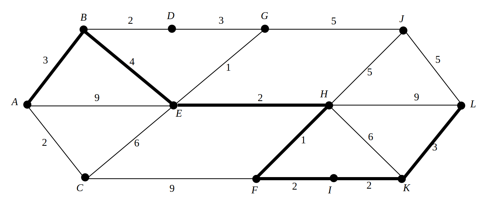
Figure 2.46: A graph taken from Introduction to Graph Theory, Fourth Edition, Wilson R.J., 1996.

Finding the shortest path between two places on a weighted graph is actually not a difficult problem. A number of algorithms have been devised for solving this problem, the most famous of which is likely Dijkstra’s algorithm. This algorithm works by finding the shortest path to the target from all locations, starting from the neighbours of the final target.

Dijkstra’s algorithm is extremely quick to run on a computer and is used as a pathing algorithm inside a very wide range of computer games as well as to many other applications.

2.12.1 Adjacency Matrix of Weighted Graphs

When using weighted graphs with computers the natural way to store the information about the weights on the edges remains to use matrices.

Consider the following graph:

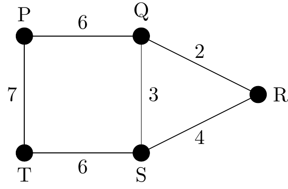
Figure 2.47: A graph to illustrate an adjacency matrix for a weighted graph

The weighted graph presented in Figure 2.47 has \(5\) vertices and the values written half-way along the edges are the corresponding edge weights.

There are then two matrices of use when studying this graph, first the standard adjacency matrix:

\[ A = \begin{matrix} & \begin{matrix}P&Q&R&S&T\end{matrix} \\ \begin{matrix}P\\Q\\R\\S\\T\end{matrix} \hspace{-1em} & \begin{pmatrix} 0&1&0&0&1 \\ 1&0&1&1&0 \\ 0&1&0&1&0 \\ 0&1&1&0&1 \\ 1&0&0&1&0 \end{pmatrix}. \end{matrix} \]

However, it is also possible to capture both the edges and their weights in a single matrix. For this purpose the following weighted adjacency matrix is used:

\[ A = \begin{matrix} & \begin{matrix}P&Q&R&S&T\end{matrix} \\ \begin{matrix}P\\Q\\R\\S\\T\end{matrix} \hspace{-1em} & \begin{pmatrix} 0&6&0&0&7 \\ 6&0&2&3&0 \\ 0&2&0&4&0 \\ 0&3&4&0&6 \\ 7&0&0&6&0 \end{pmatrix}. \end{matrix} \]

It is easy to see that this second matrix contains more information, and the first matrix can be derived from it by replacing all non-zero values with ones. For this reason this latter matrix is the one usually used in calculations regarding such graphs.

We mention this because there is an opportunity for ambiguity here. We have included multigraphs in our studies and this latter matrix could also be used to represent a standard multigraph with a lot of parallel edges. Hence it is important to always know what type of graph is being considered when looking at an adjacency matrix representing a graph.

2.13 Isomorphisms between Graphs

This is a highly theoretical topic and very difficult to study for graphs with large numbers of vertices.

(First the formal, but way too technical mathematical definition, which no doubt contains some symbols you may not have come across before!)

Technical definition of isomorphism

Graphs \(G\) and \(H\) are said to be isomorphic (essentially the same graph) if there is a one-one and onto function \(\Phi\) satisfying,

\[ \Phi: V(G) → V(H) \text{ such that edge } \{A, B\} \in E(G) \] \[ \Updownarrow \] \[ \text{edge } \{\Phi(A), \Phi(B)\} \in E(H), \]

where,

• \(E(G)\) and \(E(H)\) are the lists of edges in \(G\) and \(H\) respectively;
• \(\Phi\) is just come function which pairs up vertices between \(G\) and \(H\), denoted \(V(G)\) and \(V(H)\) respectively; and
• \(\iff\) means if and only if.

In much plainer English here is an easier to understand definition:

Friendlier definition of isomorphism

Two graphs \(G\) and \(H\) are said to be isomorphic if

There is a way to match up (i.e. pair up) the vertices of \(G\) and the vertices of \(H\) in such a way that the number of edges joining any two vertices in \(G\) equals the number of edges joining the corresponding vertices in \(H\).

Finally, the friendliest version yet:

\(G\) and \(H\) are isomorphic if there is a way to label (they might change, they might not) the vertices of \(H\) to match those of \(G\) after which the graphs \(H\) and \(G\) have the same adjacency matrix.

Example 25

These graphs \(G_1\) and \(H_1\) below are isomorphic.

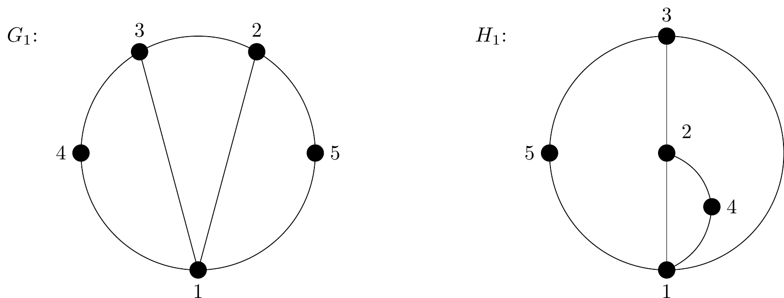
Figure 2.48: Two isomorphic graphs, \(G_1\) and \(H_1\) respectively

We normally need to think up a way to rename the vertices of one graph so that its adjacency matrix matches that of the other graph. But in this case, it turns out that the existing names already work!

One shortcut to this is to start by looking at the degrees of the vertices, since they will need to match after renaming.

Here is the adjacency list for \(G_1\):

Vertex	Adjacent vertices	Degree
1	2, 3, 4, 5	4
2	1, 3, 4	3
3	1, 2, 5	3
4	1, 2	2
5	1, 3	2

So the degree sequence is \((2,2,3,3,4)\).

Looking carefully at \(H_1\) we see that the vertices as originally named have exactly all the same adjacent vertices, so \(G_1\) and \(H_1\) already have identical adjacency matrices and so are isomorphic.

You may like to think of this whole idea as an answer to the question:

Can I relabel the vertices, and move them around so that these two graphs looks identical?

Example 26

Consider the following two graphs:

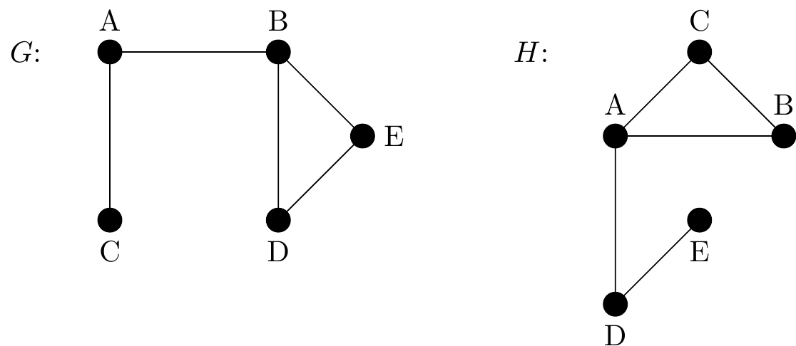
Figure 2.49: Two isomorphic graphs, \(G\) and \(H\) respectively

Here if we rename the vertices as follows:

G Vertex	H Vertex
A	D
B	A
C	E
D	B
E	C

Then the two graphs becomes identical (they have the same adjacency matrix), so \(G\) and \(H\) are isomorphic.

Example 27

One way to show graphs are not isomorphic is just to illustrate that they have different degree sequences. This is because renaming vertices has no affect upon the degree sequence. So you cannot turn one degree sequence into another just be renaming the vertices. With different degree sequences the adjacency matrix row sums are bound to be different so the matrices themselves must be different.

The graphs \(G\)₂ and \(H\)₂ below are not isomorphic as they have different degree sequences.

One final bonus topic, combines our work in Section 2.9 and Section 2.13 with a bonus new definition.

A subgraph \(G'\) of a graph \(G\) is a new graph which is derived from \(G\) by removing any number of edges and vertices from \(G\), but adding nothing new.

Removing a vertex removes all edges that are incident to it.

Practice

Find a subgraph of \(G\) in Figure 2.49 which is isomorphic to \(C_3\).

Can you find a subgraph of \(G\) in Figure 2.49 which is isomorphic to \(C_4\)?

2.14 Vertex (Graph) Colouring

The most well-known graph colouring problem is the Four Colour Problem which was first proposed in 1852 when Francis Guthrie noticed that four colours were sufficient to colour a map of the counties of England so that no two counties with a border in common had the same colour. Guthrie conjectured that any map, no matter how complicated, could be coloured using at most four colours so that adjacent regions (regions sharing a common boundary segment, not just a point) are not the same colour. Despite many attempts at a proof it took until 1976 when two American scientists, Appel and Haken, using graph theory, produced a computer-based proof to what had become known as the Four Colour Theorem.

In graph theory terms vertex (graph) colouring problems require the assignment of colours (usually represented by integers) to the vertices of the graph so that no two adjacent vertices are assigned the same colour (integer).

A \(k\)-colouring of a graph is a colouring in which only \(k\) colours (numbers) are used.

The chromatic number for a graph is the minimum number of colours (numbers) required to produce a vertex colouring of the graph.

The chromatic number of a graph \(G\) is denoted by the Greek letter \(\chi(G)\) (chi).

A graph with no edges has chromatic number 1 since you colour every vertex the same colour and none of them are adjacent!

The complete graph \(K_n\), however, has chromatic number \(n\), can you see why \(n-1\) is not enough?

Identifying the chromatic number in these two cases is straightforward. In general, however, determining the exact chromatic number of a graph is a hard problem and no efficient method exists. The only approach that would identify the chromatic number of a graph \(G\) with absolute certainty would involve investigating all possible colourings. Clearly as graphs become larger this method becomes impractical, even using the most powerful computers that are available. The best that can be done is to determine lower and upper bounds on the chromatic number and techniques such as looking for the largest complete subgraph in \(G\) (for a lower bound) and the Greedy algorithm (for an upper bound) enables us to do so. The Greedy algorithm however is very inefficient but is adequate for ‘small’ graphs with the aid of a computer.

Example 28

We shall colour this graph with the minimal number of colours.

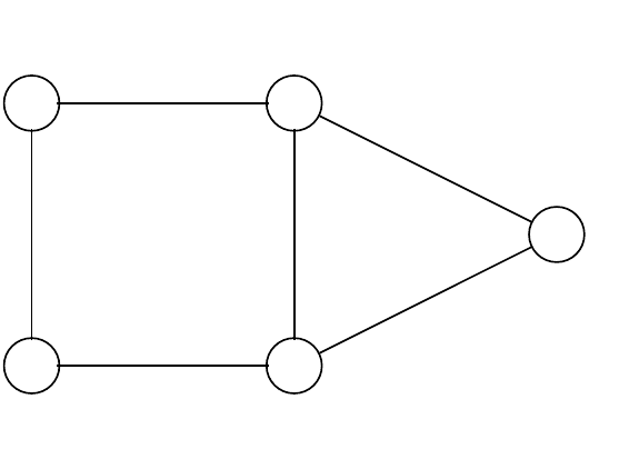
Figure 2.50: A graph to illustrate chromatic number

First an actual colouring, using colours and then using integers:

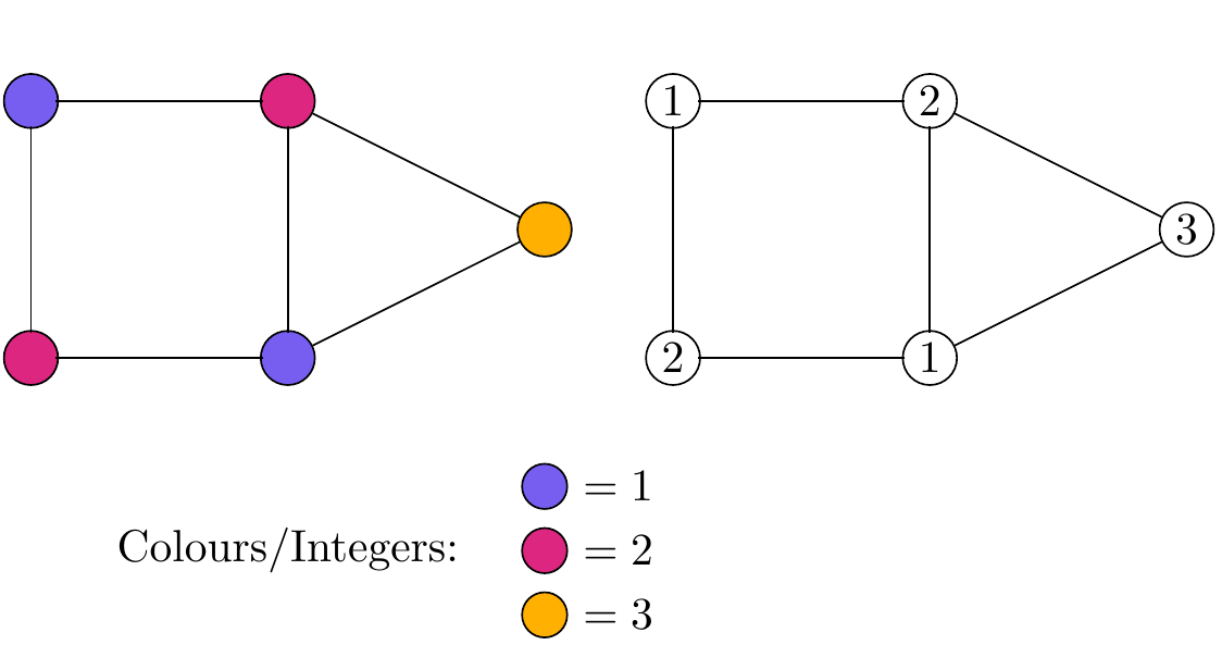
Figure 2.51: Vertices of Figure 2.50 coloured with just 3 colours and then coloured with three integers.

These illustrations show how to label the vertices using just three distinct colours/integers in such a way that no joined vertices share a colour/integer.

With some thought you can appreciate that it cannot be done with only 2 colours. Hence for this graph \(G\) the chromatic number is \(3\), i.e. \(\chi(G)=3\).

Practice

Try and colour the vertices of the following graphs (i.e. label the vertices of the graph with as few different numbers as possible so that no two adjacent vertices have the same number)

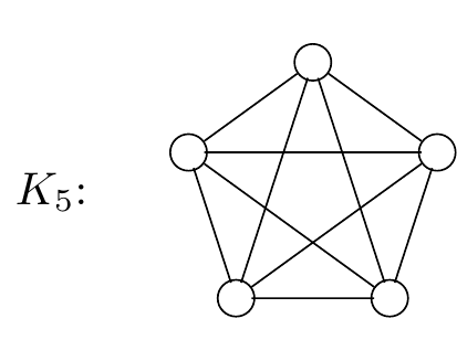
Figure 2.52: \(K_5\) ready for colouring

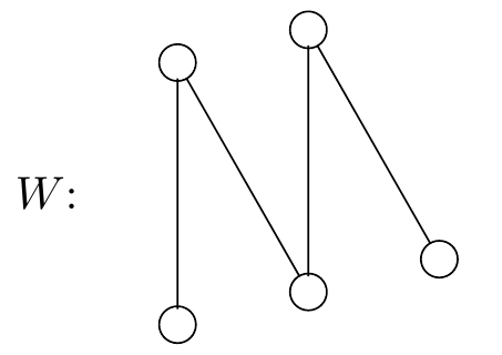
Figure 2.53: A W-shaped graph ready for colouring

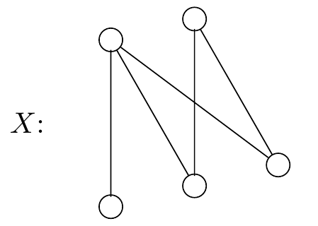
Figure 2.54: Another bi-partite graph ready for colouring

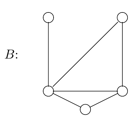
Figure 2.55: A more difficult graph to colour

2.15 Summary

This unit has provided an introduction to the important topic of graph theory and you should now be able to:

• identify different types of general graphs including: undirected and directed graphs, simple graphs and multigraphs.
• understand basic terminology associated with graphs, including: connected, vertices, edges, arcs, adjacent, incident, degree sequence, in-degree, out-degree, etc.
• identify different types of specific graphs: regular graphs, complete graphs, cycle graphs, bipartite graphs, tree graphs and weighted graphs.
• state the Handshaking Lemmas for both undirected graphs and digraphs.
• identify walks trails and paths on undirected graphs and digraphs.
• determine whether or not a graph (undirected or digraph) is Eulerian and identify an Euler circuit if one exists.
• determine whether or not a graph (undirected or digraph) is Hamiltonian and, for “small” graphs, identify a Hamiltonian cycle if one exists.
• construct adjacency matrices for undirected graphs and digraphs.
• construct an undirected graph or digraph given an adjacency matrix.
• understand what is meant by isomorphic graphs.
• understand what is meant by a graph colouring and the chromatic number of a graph.