02
-
Data organisation and some basic relational ideas
- In this week, we will cover the following topics:
- Data: that you can design the structure of data, including the relationships between data.
- The important of being able to uniquely identify datum within a set of data.
- How to accumulate relationships between data, as data, stored in tables.
- A brief look at a real word set of data known as Codepoint, and the limitations.
- ‘Programming’: the distinction between declarative programming and algorithmic
- … and will result in the following learning outcomes:
- An initial appreciation that it is good to be systematic in how data is represented.
- That data ‘keys’ allow us to access specific datum.
- Knowledge that tables can be used to store data and relationships between data.
- That real-word data is available, but not necessarily perfectly organised.
- A feeling for the kind of programming relevant for database interactions.
-
2.1 Designing for data
2.1.1 Relationships between data/datum
- During week 1, we discussed the idea of a ‘legacy’ data management system, seen as a consequence of there being no enforced rules for data entries.
- The order (we have seen that this has important aspects to it concerning the actual delivery) has other important information attached to it. Namely, the order relates a product to a customer. We might think of this situation, then, as two physical entities (Product and Customer) being connected by an ‘event’, the ‘order’:
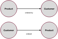
- Customer ‘ordered’ Product.
- Product ‘ordered by’ Customer.
- Figure 1: Basic relationships seen both ways
- Consider an associated data entry example, not for data entered into a spreadsheet, this time, but through a website; here we might imagine a retailer website form designed to receive data concerning the customer.
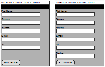
- Figure 2: Website mock-up examples for ‘new customer’ website form.
- We present two choices (see Figure 2). The first choice is designed to receive 5 entries, i.e.., First Name, Surname, Address, E-mail, and Tel (short for telephone number). The second choice is designed to receive 6 entries, i.e., First Name, Surname, Address, E-mail, Tel, and Product. We do not need to question the design of the forms themselves. The forms, for our current purposes, merely provide an interface through which data is input to ‘the system’.
- Let us take a look at what the actual data might ‘look like’ (in storage), after a company has had a number of new customers added. We will assume that the second form was adopted by the company, the one with all of customer details, in addition to the first customer-chosen Product.
First_Name Surname Address E-mail Tel Product John Davis Salmon Road jd@cloudme.com 077**08 Soap Powder Aileen McManus East Avenue am@lmail.com 0131**9 Table David Smith North Close jd@wohoo.com 0141**1 Wood Polish Sarah Jones Queen Road jd@geewizz.com 0131**9 Nails - Table 1: Accumulated customers.
- From the point of view, a customer’s first order, maybe this kind of data makes sense? If you look on most retail websites, however, you will find that the customer is required to register an account separately to the order. Nevertheless, as we mentioned, we are not concerned here about the design of the web interface, although the following issues are worth highlighting in relation the above example:
- 1. What happens if a customer, named John Davis, registers himself, ordering the product Soap powder, as above, then three months later somebody else with the same name registers and orders a Bike?
First_Name Surname Address E-mail Tel Product John Davis Salmon Road jd@cloudme.com 077**08 Soap Powder Aileen McManus East Avenue am@lmail.com 0131**9 Table, TV David Smith North Close jd@wohoo.com 0141**1 Wood Polish Sarah Jones Queen Road jd@geewizz.com 0131**9 Nails John Davis West Close jd@cloudme.com 077**08 Bike - Table 2: Customer table version B – non-unique names.
- 2. How well does the Product column ‘cover’ the relevant data now and in the future?
- Point 1: Assuming that this does happen, if one of the ‘John Davis’ customers then orders a Table, how do we know which John Davis this is? Perhaps we can identify them uniquely by their phone number or e-mail address?
- Point 2: If we look again at the table, during the time the second John Davis registered, Aileen McManus ordered a TV. Is storing the collection of products in this way acceptable? It certainly does not seem consistent. The original meaning of the Product category was initial Product.
-
2.1.2 Two initial problems
- Although we are now looking at a different example, one involving a hypothetical web-based system, we are stuck in the same sort of file-based, spreadsheet mind-set introduced in week 1, but we have introduced two new problems:
- 1. The problem of allowing unique access to a set of data.
- 2. The problem of how to best represent accumulative changes / additions to data, but without allowing structural changes to be made i.e., without allowing change to the overall structure of the data itself.
-
2.2 Relational solutions to the problems
- As a way of introducing some of the basic ideas of relational databases, we will now re-design how our data is stored, expanding the examples above, to address our two initial problems.
- Let us make the data a little bit more believable, even if not necessarily ‘realistic’. For example, a retailer is likely to have a larger set of data that relates to a specific Products; what is important from a customer-facing point of view – the name of the product – would then be one column in this larger set of values.
- Examples of what might be important to the retailer:
- Where the product comes from – the Supplier.
- The unit cost of purchase – PurchaseCost.
- The unit price at point of sale – SalePrice.
- Product code – ProductCode.
- Product category – Category.
- Product name – Product.
ProductName Category ProductCode SalePrice PurchaseCost Supplier Soap Powder Home 02147698 4.50 2.50 15 TV Electrical 05070012 999.99 650.00 05 Table Furniture 08608376 299.00 100.00 09 Wood Polish Home 02447701 2.50 1.00 11 Nails Hardware 01570627 3.00 50.0 15 Bike Leisure 09377700 680.00 400.00 155 - Table 3: Products
-
2.2.1 Unique identification
- We are now going to re-define Table 2 (Customer table version B). We do this to provide a unique identifier for each customer, which we will call CustomerId, and we maintain all of the other columns as defined previously, in Table 4 (assume that the E-mail entries exist – they are omitted for ease of visualization).
CustomerId First_Name Surname Address E-mail Tel ProductName 0001 John Davis Salmon Road . 077**08 Soap Powder 1298 Aileen McManus East Avenue . 0131**9 Table, TV 0032 David Smith North Close . 0141**1 Wood Polish 0099 Sarah Jones Queen Road . 0131**9 Nails 9834 John Davis West Close . 077**08 Bike - Table 4: Customer table version C
- You might have noticed a potential problem with the ProductName column in Table 2 and Table 5. Again, there is potential for the products to ‘overlap’ in terms of the ProductName column – the names are, again, too generic to act as unique identifiers. For example, a customer might choose between many different kinds of Soap Powder, so, we cannot use such product names as unique identifiers (they are not unique!).
- There are two rules for unique identifier’s:
- They must be unique!
- They should not change value!
- This is why it is a bad idea to use a phone numbers or e-mail addresses as unique identifiers.
- Therefore, in order to uniquely identify a customer, we use the CustomerId. In order to uniquely identify a product, we use the ProductCode. The unique identifier is simply a value that is used that is unique to a given row (rows within a given table cannot have the same unique identifier). The phrase ‘unique identifier’ an accurate description, is also referred to as the ‘primary key’ because it provides primary means of row-wise access to data.
- Relational databases: key definitions
- Schema: the entire structure and description of data. Importantly, the schema is thought of, and packaged, as part of the database. In this way a database is ‘self-describing’.
- Primary key: the column attribute of a table, whose row value is unique in the set of rows.
- Table: the axiomatic representational form employed in relational databases
- Row: accumulative
- Columns: schematic
- Relations: typically, the ‘links’ made between datum. In the area of relational databases, collections of such relations are represented as tables.
- Tuples: a set of data that is ordered according to the colums. Any given row defines a tuple. If the number of colums is n, then each row is an n-tuple. So, each row in Table 4 is an 7-tuple, whereas each row in Table 3 is an 6-tuple.
- Attributes: Refer to the set of columns in a table; these are thus the tables attributes and at the same time the attributes of each row of data.
- Entity type: the specific name given to an entity, which is essentially a collection of columns/tuple etc., associated with that type.
- Table 5: Some key, definitions regarding relational databases.
-
2.2.2 Accumulating relational data
- In the previous subsection we solved the problem of unique identification of data by defining, and giving an example of, the use of primary keys. Now we will show how to store relations between data in the style of the relational approach.
CustomerId ProductCode Date 0001 02147698 02-01-2016 9834 09377700 02-02-2016 0032 02447701 23-02-2016 1298 08608376 05-03-2016 1298 05070012 05-03-2016 0099 01570627 21-03-2016 0032 08608376 19-03-2016 0032 01570627 19-03-2016 . . . Table 6: Ordered table. - Note that the second problem of storing numerous products per-customer is, also, easily solved by this table; we simply add a new row each time an order is placed – no need to add the new product to the same row as other products. Accumulative changes are represented without structural changes being made to the table, such as adding a new column for a new product.
- In Figure 3 we present (on the left) a representation of the relationships specified by Table 6, along with the tables that contain the primary keys. Notice that the circles in Figure 3 contain the values of attributes pertaining to the primary keys. In other words, we have chosen a readable-friendly attribute of each row indicated by the primary key, rather than to represent the primary keys themselves. This is a little bit like saying:
- Select from the Customer table the First and Second Name according to the CustomerIds in the Order table.
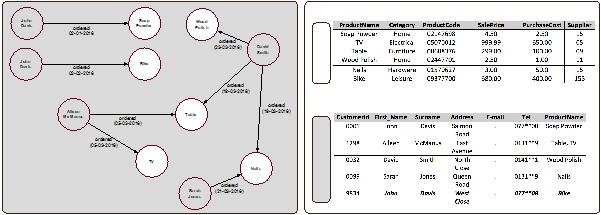
Figure 3: A view of what a relational table represents. -
2.3 A real-world, file-based data set: Code Point@ Open
- Instead of working with ‘fake’ data for illustrative purposes, in this section we are going to take a look at a real-world data set. The data set is the set of UK postcode data known as Code-Point® Open (Ordinance Survey, 2015). Postcodes are grouped combinations of numbers and letters, which are associated with a postal area. An example post code is:
- G4 0BA
- The ‘G’ part of the postcode stands for Glasgow. The ‘4’ part of the postcode represents an area in Glasgow, and the 0 represents an area within the area of area ‘4’. So, as we read across the string G40BA we effectively ‘zoom-in’ to quite a small region. Postcodes are used to deliver letters, and are used to sort mail, to make the delivery of mail more efficient. Imagine if a postman were to randomly deliver letters in the UK. They would, for example, deliver a letter in Birmingham, followed by one in Aberdeen, some 680 kilometers North! So, postcodes help sort mail, which in turn helps organize its efficient delivery. A list of the general postcode areas is available on wikipedia.org:
- https://en.wikipedia.org/wiki/List_of_postcode_districts_in_the_United_Kingdom
- We will see later in the course that postcodes, and the associated data within Code-Point® Open, along with some other technology we introduce later, can be useful for other things, too.
- For now, though, we want to focus on the data, to see how it is structured and to see what we might want to do to put it into a database. Firstly, Code-Point® Open can be downloaded from:
- https://www.ordnancesurvey.co.uk/opendatadownload/products.html
- Code-Point® Open (Ordinance Survey, 2015) is an almost-comprehensive list of the entire set of postcodes in the UK. That is, it has the whole of the UK’s postcodes listed, excluding Northern Ireland. The database contains approximately 1.7 million UK postcodes, with some 25 million adjoining addresses; therefore, each separate postcode serves about 15 post address, on average (15 x 1.7 = approx. 25).
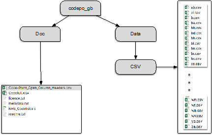
- Figure 4: Structure of codepoint open directories.
- The data is distributed by the Ordinance Survey as a set of files. In Figure 4, we present the structure of the folders and where the data files etc. can be found. The top-level folder is <codepo_gb>, which contains two subfolders, <Doc> and <Data>, and inside <Data> we have the folder <CSV>.
- We are only interested in the ‘.csv’ files. The ‘.csv’ postfix stands for comma separated values, and ‘.csv’ files are typically text files, which can be opened in any standard text editor. Most of the files are contained in the <CSV> directory:
- codepo_gb/Data/CSV/*.csv: this set of 120 files (the three asterisks ‘*’ in Figure 4 hide 102 files that fit, alphabetically, between <ca.csv>, <wn.csv>) contains the actual data.
- But there is another .csv file here:
- codepo_gb/Doc/Code-Point_Open_Column_Headers.csv: this single file defines the headers to the data
- Given the structure of some of the public data that is available (which can be very messy), we should be reasonably happy with this file-based organization of Code-Point® Open. Of course, there is the problem that the data is stored into files, and if we wanted to create a program that needed to use postcodes, the files would take a long time to read into memory. However, the files are relatively well organised.
PC PQ EA NO CY RH LH CC DC WC - Table 7: Non-verbose Code-Point® Open header/column fields.
Postcode Positional_quality_indicator Eastings Northings CY RH LH CC DC WC - Table 8: Verbose Code-Point® Open header/column fields.
- Let us take a closer look at the header file. This file contains 10 ‘columns’ and 2 ‘rows’. In the text file, the way that the columns are coded are by the insertion of the comma ‘,’. The rows are just specified by being placed on separate lines, using on the keyboard the <Enter> key. The way ‘enter’ is coded in a text file is by using ‘/n’ (this is not necessarily visible in text editors), which is otherwise known as the carriage return. The header/column fields are presented in a relatively non-verbose way in Table 7, whereas Table 8 contains relatively verbose labels. Don’t worry at the moment what these fields mean – we are not even interested in knowing what all of this means, but we will look at the most important (from our point of view) fields in an example of the data.
- So, the first columns contain the actual postcode. Then, there is somethings known as the positional quality indicator, followed by entries for the eastings and northings. Let us take a look at an extract from a data file see in Table 9.
"G4 0AJ",10,260044,665214,"S92000003","","S08000021","","S12000046","S13002649"
"G4 0AL",10,260044,665214,"S92000003","","S08000021","","S12000046","S13002649"
"G4 0AN",10,259725,664965,"S92000003","","S08000021","","S12000046","S13002649"
"G4 0AP",10,260044,665214,"S92000003","","S08000021","","S12000046","S13002649"
"G4 0AQ",10,260044,665214,"S92000003","","S08000021","","S12000046","S13002649"
"G4 0AX",10,259349,666274,"S92000003","","S08000021","","S12000046","S13002650"
"G4 0BA",10,259296,666080,"S92000003","","S08000021","","S12000046","S13002650"- Table 9: Extract from file <codepo_gb/Data/CSV/g.csv>
- Look at how designers of the data have decided to represent different types of data within each column. They define a String type in the file by enclosing with double quotations “”. For example, the right-hand column in the final row (SI3002650) is a String type by virtue of the fact that it is represented between the commas as “SI3002650”. On the other hand, numbers are stored as is, without being enclosed with quotes.
- Let us take a look at some example numbers and what they represent, taking the yellow-highlighted line as an example. This row is the entry for the G4 0BA postcode, mentioned above, which is the postcode for Glasgow Caledonian University. The ‘positional quality indicator’ (column 2) has a value of 10, the ‘easting’ (column 3) a value of 259296, and the ‘northing’ (column 4) a value of 666080. Eastings and northings are a form of geographical coordinate. Therefore, a location on the surface of the earth can be found with an <easting, northing> pair.
- So let us check how accurate the easting northings data is. Perhaps we can use a leading maps provider to do this? Not necessarily! If we plug these into Google Maps we will get an error, because Google maps (and many other web services come to that) represent geo coordinates differently, using the Latitude and Longitude. Nevertheless, it is possible to check the information by using a web site (http://www.gridreferencefinder.com) coded to handle <easting, northing>-style coordinates. If you go to this site and enter the values, the a pin will be dropped inside the boundary of the GCU campus! Indeed, as we see in Figure 5, the coordinate <259296, 666080> is situated at a specific point within the campus, actually just next to the Saltire Centre, which is one of the universities focal points for learning.
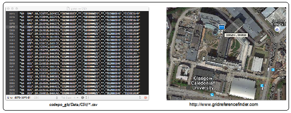
- Figure 5 The GCU postcode.
-
2.3.1 A critique of Code Point@ Open
- We are not interested here in critiquing the actual raw data as a resource. As we have mentioned, the resource is very valuable in itself. We do, however, want to briefly reflect on: the folder/file structure of the resource, and the structure of the raw data itself.
- Strictly there is no ‘right’ way to structure a data resource, but you should try and notice some inconsistencies with the organization of the files. Take a look again at Figure 4. For example:
- 1. Reflecting on the folder/file structure of the resource:
- a. The file <codepo_gb/Doc/Code-Point_Open_Column_Headers.csv> contains the headings of the data. Should this not be part of the data itself, perhaps kept inside the codepo_gb/Data folder somewhere? Furthermore, this file has an ‘.csv’ extension. Why, then, is it not in the CSV directory?
- b. Metadata is data about data. It is, therefore, data. Why is codepo_gb/Doc/metadata.txt not in the Data directory then?
- c. All of the files in the Data directory are ‘.csv’ type files. Is the naming of this folder redundant?
- 2. The structure of the raw data itself:
- a. As mentioned, Strings require additional coding (“String”) within the data file itself! Shouldn’t the type of the data be declared outside of the actual raw data entries? The answer to that is yes.
- b. How do we write an application program to get a specific data entry, or set of entries, out of a file, or set of files? And how do we do this quickly? The answer to this is that it can be quite cumbersome to code access to specific values. The algorithms required to do this need coding in the application. Furthermore, reading files from disk is inherently as slow procedure.
- Many of the issue we mention here, concerning file-based representations, simply seem to disappear when using databases because we are working within the well-defined constraints of a database.
-
2.4 ‘Declarative’ programming v ‘Algorithmic’ Programming
- Before we finish this week, we want to pick-up on point 2b, and on the fact that in writing an application program we would need to write algorithms that provide access to the data, or use someone else’s code that does this. Table 10 provides a very simple algorithm, and one that would potentially be very slow, to access the easting and northing data from the file <g.csv>. Table 11 provides the equivalent database style declaration designed to retrieve the same data from a database. An important point to note is that Table 10 is a highly simplified set of pseudo code, whereas Table 11 is the full MySql statement, which if you ran within a database environment would actually work.
- We will see later on in the course, using a programming language known as Java, that within application programs you can run Sql statements. Rather than writing application code to access a file based system, running Sql statement/queries exposes all of the advantages of databases to the application program.
Program style code // Create a file instance in memory from g.csv File f = new file(“g.csv”); // Open the file g.csv f.open(); // Access line G4 0BA for each line in the file { if (line elemetn 1 is equal to G4 0BA) { targetLine = current_line } } // Get the information you want from that line Easting e = targetLine.getElemtn(3); Northing n = targetLine.getElemtn(4);- Table 10: Application program pseudo code to retrieve data from file.
Database style declaration

// Select required data from the database
Select Eastings, Northings from database where Postcode like ‘G4 0AB’;
- Table 11: Code to retrieve data from file v database declaration.
- What is the basic difference between algorithmic programing and declarative programming?
- Algorithmic programming: here the control (and therefore the responsibility) and the design of the algorithms are in the hands of the programmer. All of the steps need defining and implementing in-code. This can be a highly rewarding process as the programmer designs code for re-use, or speed, or some trade-off between the two.
- Declarative programming: this is not ‘programming’ in the same sense. A declarative ‘programming’ language states which data is needed, from which database. The enjoyment of working with databases is often related to the comparative simplicity of retrieving data from a database as compared with having to access it from a file-based system, but is also related to the process of actually designing the structure of the data itself.
- Either form of programming is no sense better than another. As we have suggested, the two styles of programming are absolutely complementary.
- Own creativity and resourcefulness. You might, not yet, be capable of implementing your ideas, but, if you work hard, then this will come with time.
-
2.5 Summary
- Database development should not just be undertaken by jumping straight into creating a database. Important processes of design must take place first.
- We introduced the relational approach and listed some basic relational database definitions.
- We then considered real-world file-based dataset known as Code Point Open. The reason we did this, was to develop an appreciation for an existing File-based system, and the often-used comma separated values (.csv) format.
- We then considered how we might write a program to access the data within such a system.
- This led us to the important distinction between declarative programming and algorithmic programming. Query languages are very much based on the idea of declarative programming.
- Download PDF Version