03
-
Relational Data Modelling I: modelling processes and the language of sets.
- In this week, we will cover the following topics:
- What modelling is, and specifically what data modelling is.
- What data modelling involves in real-world situations (modelling cycle)
- Some visual design conventions used in relational database design.
- The language of sets
- … and will result in the following learning outcomes:
- An understanding of the general modelling cycle and how database designers might liaise with business clients.
- An appreciation for the fact that good design needs a good appreciation of the data domain, and the data in the domain.
- An understanding of the mathematical language of sets.
- An appreciation that understanding this language will help inform database queries.
-
3.1 Models and modelling processes
- The same kinds of words can be used in different contexts and, consequently, take on slightly different meaning. Therefore, it is important to distinguish what we mean by modelling and distinguish the meaning we are using in the context of databases. We will do this by contrasting with a slightly different, but commonly-used, notion of modelling.
-
3.1.1 What is modelling?
- Generally, a model is a representation of something in the real-world, designed to capture the essential aspects of that ‘thing’. At a concrete level we might, for example, consider a child playing with a model/toy boat because they have developed an interest in real boats. Similarly, a marine architect might build more realistic features of boats into a more advanced model (physically built, or coded into a computer) of a real vessel and, furthermore, might test the design according to conditions of a simulated environment (physical wave machines, computer simulations of sea conditions).
- In academia, equational models are often designed to capture features of the physical world, in the form of equations. Equations then can be used to analyse the behaviour of the real system, analogously to how a physical model of a boat might be used to understand ‘boat’ behaviour when, scaled-up in size, built to cross the ocean. Equations can capture physical systems of varying abstraction. For example, Newton’s laws of gravity describe the force interactions between objects that have mass, whereas more concrete models might be concerned with specific forces, in an application of Newton’s laws, to identify the required strength of a ships hull, for example. For all such models a useful rule of thumb, attributed to Albert Einstein, is that the model should be simple, but not too simple: “Everything should be made as simple as possible, but not simpler”. The important aspect of modelling identified by Einstein is that there is little point in having a model that is very simple, if it does not properly describe the real-world situation. On the other hand, a model that is overly complicated will not serve to organise our understanding, either. A balance must be struck.
-
3.1.2 What is data / database modelling?
- As the title of this week suggests, we are interested in relational data modelling, specifically, extending our less formal introduction to this area, covered in the previous week (week 2). The reason we have briefly considered the above meaning of modelling, commonly used in academia and science, is to distinguish it from the specific meaning of modelling that concerns us in this course. As Ritchie states:
- “In the study of databases, our interest is in data modelling. The role of data modelling is to provide techniques that allow us to represent, by graphical and other formal methods, the nature of data in real-world computer applications. The principal justification for the use of data modelling is to provide a clearer understanding of the underlying nature of information and the processing of information.”
- Ritchie (2002, p19).
- Read the last sentence of the Ritchie quote again: “The principal justification for the use of data modelling is to provide a clearer understanding of the underlying nature of information and the processing of information”. You could just as easily substitute the word ‘information’ for ‘data’, and we probably should: in other areas of computer science and computer engineering, ‘information’ means something more distinctive and relates to the amount of surprise in the flow of data (as binary digits) through cables, which is captured by Shannon’s law, a highly pragmatic and important equation in the subject area of computer networks.
- Nevertheless, you should infer from Ritchie’s quote the emphasis on formality and during this week we will become more formal in the way we start to describe. Hence, we start to develop a language of relational data modelling. Fortunately, relational database models are quite straightforward to understand.
-
3.2 The process of database design/modelling
- Before we begin to properly learn the language – the tools, (graphical and other) descriptions, concepts, methods etc. – of relational data modelling, we will introduce the practical steps that typically take place during the early-stage process of database development. Of course, the actual steps that take place will vary according to the specific application domain. Nevertheless, even caricaturing this process somewhat will give us a feel for this important aspect of database development. Remember the title of this course is Database Development and, while it is important to learn the appropriate technical languages, we always need to remember their practical context and purpose.
-
3.2.1 What is database development
- As with many aspects of software development, an ability to develop useful software depends on the developer requiring a knowledge of the problem domain, and in database development this means developing a view of the data, based on what the database will be used for and the best way in which data can be accessed and stored efficiently for these purposes.
- The domain, i.e., the target for the data modelling exercise, of course, contains the target data. As we have discussed previously, this data might be stored as a file-based system. It is important, for the developer, to understand how the data is understood from the point of view of the current user of that data, in the context of the client business, for example. The data will be used within this context in a certain way and, consequently, the user will have developed a view of the data – this will include how the data is related, stored, used, updated etc. In order that a useful database representation of the data can be developed, it is important during the initial stages, as with software development more generally, for the developer (in this case the database developer, or database development team) to get a good understanding of how the client understands and uses the data, as well as developing a knowledge of the current storage and representation of the data itself. In order to develop this understanding, questions should be asked to facilitate this and, again as with software development generally, client interactions will be quite frequent during the initial stages.
- When the database team begin to implement the database it is a good idea that the data modelling is complete. That is, for relational database design development is done in a top-down fashion. The phrase top-down, here, refers to the idea that thorough comes first, before the database is implemented. In recent times, the idea of agile software application development has taken hold, which emphasizes a modern approach to development, in contrast to the more traditional, top-down approaches to software engineering. However, an agile mind-set is not best suited to relational database development. This is a view well expressed by Allardice (2015):
- “…planning is vital [for relational database development]. Whereas in other areas of development such as agile incremental approaches (build something quickly, get it out there, revise it, add new features [quickly] over weeks or even days), relational databases reward up-front planning because the entire point is to impose rules, constraints and structure on the data and we don’t want to have one set of rules for one week and another set of rules for another week.”
- Allardice (2015)
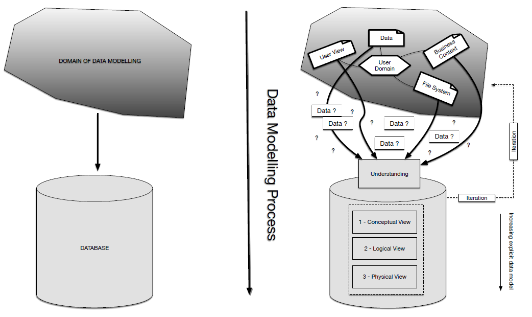
- Figure 1: Database modelling
- Therefore, the database modelling process itself is about how we get from the user-defined view of the data, how the data gets processed and updated etc., to the associated, database view of the data
-
3.2.2 3 key steps: processes of data model development
- Figure 1 presents a schematic, which helps visualize the intended process of moving from the application domain to the design of the database itself. Note well, there are three main steps during the database development process. These stages all concern the process of identification and specification of entities and relationships between entities from the data. Each level, from 1 to 3, is intended as a phase of identification, each step being followed by another one, which adds details and specification, such that the data model becomes more and more explicit over time.
- 1. Conceptual data modelling (least detailed): this is to identify the salient entities within the data and the most important relationships between them. Given that two entities have been identified (say, Customer, and Product), for example, we know that these two entities are related in some way. At this stage it is typical to remain quite high-level in our descriptions from the point of view that we do not need to disclose all of the detail. For example, we only really need to know that Customers and Products are entities; there is no need to go further by being explicit about Customer and Product attributes – e.g., ‘Customer Number’, ‘FirstName’, ‘Surname’, ‘Address’, etc., or for product ‘ProductNumber’, ‘ProductName’, ‘Category’.
- 2. Logical data modelling (more detail): progressing from the previous stage, we start to identify all of the entities in the data model, and all of the relationships. For each entity we specify all of the attributes and identify the primary key in the data, along with the identification of foreign keys, which are used to define the relationships between entities.
- 3. Physical data modelling (fully detailed): at this stage a comprehensive model of the data is in place, in the form of a logical, entity relationship diagram. However, this additional step might include alterations to the logical model. This diagram is specified in tabular form, including all of the primary keys, relationships (foreign keys) etc.
- Steps 2 and 3 also involve something known as normalization, and possibly denormalisation. However, we do not cover or define these aspects here – we will return to this topic in a future week. Again, it is important we emphasise that the three-step process of data modelling is one of design only, no implementation.
-
3.2.3 Introduction to some visual conventions
- As in many areas of software engineering, the output of the design process – the design itself – can be communicated to others in natural language (i.e., text), but a diagram can sometimes be worth a thousand words. Therefore, just like we might use UML to communicate the design of an application program, database design comes with its own diagrammatic tools. We briefly look at commonly used diagrams here and a simple example.
- In Figure 2, we present some common graphical components typically used to construct entity-relationship diagrams. Entities are square-boxed, Attributes are represented by ovals and actions, which relate entities, are represented by diamonds. Figure 2 also contains typical line type used to denote the mapping between entities – mappings can be of various kinds (one-to-one, one-to-many, one-to-zero-or-many, one-to-one-or-many, many-to-many).
- In the example, we have three entities (Customer, Product and Order). A singular, concrete situation can be imagined as follows: a customer is browsing an on-line shopping web-site they have already created an account with. He/she clicks on a product, likes the look of it and consequently orders the product. In a similar vein, but out of sight of the customer, the customer consequently generates an order – i.e., a stored set of information, that contains the product, which is used in the end by the company to make sure the product arrives to the customer. Looking at the example we can see that these various actions relate the given entities.
- However, the purpose of the diagram in Figure 2 is not to merely represent any single situation, specific to a given customer ordering a product. The purpose is to represent all such situations. For example, take three separate situations (Situation A, Situation B and Situation C), which are all different. Situation A is the one we just described: a single customer ordering a single item, resulting in the generation of a single order that contains the product. Alternatively, in situation B, we can have a customer who has registered an account but who has placed no orders at all. Situation C is different again – customer C has visited the site many times, on occasions ordering a varying number of products at any one time, after accumulating them in their basket, then triggering one order on completion for numerous products. We therefore require the relationship between Customers, Products and Order to be well defined, meaning that the definitions of the relationships need to represent realworld use cases. The example triadic relationship between Customer, Product and Order is defined quite specifically in the diagram. In addition to the actions that connect the entities, the connections specify well-defined constrains, as follows:
- A Customer can order one or many products at one time.
- A Customer can generate one Order when purchasing their products, but over time they might accumulate many of them.
- A Product type can be ordered never, once, or many times from any given Customer
- An Order can contain one or many Products.
- An Order might never be generated by a customer (someone who only registered the account and did not buy anything), might be generated once (or many times) by other customers.
- Technical diagrams are useful to people who learn them. Although it takes time to learn their meaning, in the end this hard work will pay off. This is because diagrams then speak to the developer about the design, and in quite an efficient way (compare the amount of text written about the diagram, above, with the simplicity of the diagram itself). Over time you will learn to read diagrams quickly, and create them such they you can communicate your own creations to others as efficiently.
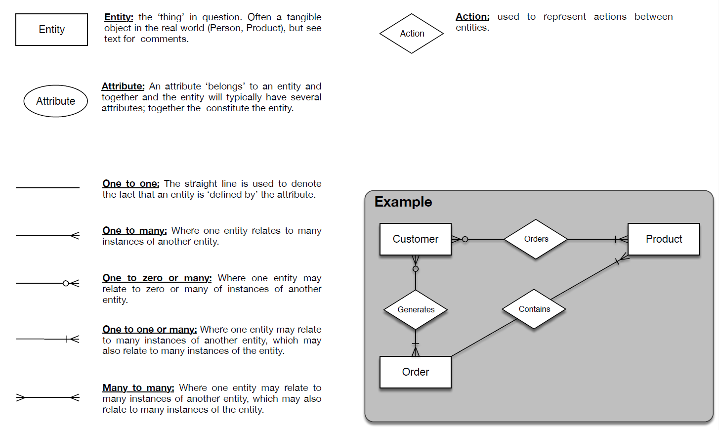
- Figure 2: Relating entities graphically
-
3.3 The language of sets
- Many textbooks have at least some reference to the notion of sets. For the beginner, these sections can quite often look intimidating, given the strange looking notion used, e.g.:
- or:
- However, this strange-looking notation, like most mathematics, is merely a form of shorthand that only looks strange, but in fact fairly easy to understand. Indeed, many concepts related to set theory are so simple that they can actually be illustrated visually, which we will demonstrate soon. The reason it is worthwhile reviewing the language of sets, apart from to put the intimidation factor in its rightful place, is because set-based operators underpin what is known as relational algebra, the theoretical foundation of relational databases and query languages. Sets therefore provide the axiomatic substrate for many of the practical things that you will do in relational database development.
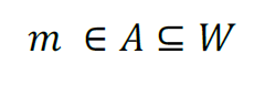
- A set is “a collection, possibly infinite, of distinct numbers, objects etc., that is treated as an entity in its own right, and with identity dependent only upon its members” (Borowski and Borwein, 1989). The members of a set thus have in common that they are members of the set, and for some reason: Kenya and Mauritius are inside the set African Countries; Scotland and Wales are inside the set United Kingdom; the iPhone, iMac and iPod are inside the set Apple Products etc. In these examples Kenya, Mauritius, Scotland, Wales, iMac, iPhone, iPod etc. are said to be members or elements of the set. Members of sets are typically denoted with lower-case letters whereas sets themselves are denoted with upper-case letters. For example: to denote Mauritius we might choose the letter ‘m’; to denote the set of countries Africa we might choose the letter ‘A’, and to denote all of the countries in the world we might choose the letter ‘W’. It is clearly the case that Africa, A, is a set of countries that is ‘contained within’ the set of countries of the world, W, and that Mauritius, m, is in Africa. Therefore, the mathematical statement:
- says “Mauritius is in Africa, which is a subset of all the countries in the world”. Hence, there is nothing mysterious about the mathematical form, once you know what the symbols mean.
-
3.3.1 Sets, visually
- Let us consider a set of objects to begin with: a bicycle, a motorbike, a car, a bus, a truck, a boat, a sailing boat, an airplane. We follow the idea that a set of objects can be thought of as being contained together inside the set, which is visually rendered as a see-through container (Stewart, 1995), such that we know which objects are there. Additionally, we denote the act of placing the objects in the container with the mapping symbol (↦). In this way, Figure 3 defines the act of creating a set of vehicles.
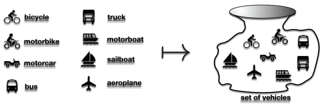
- Figure 3: Creating a set
- Although we have decided to place all of the objects into a single set, we are at the same time able to recognize that each individual member has attributes. For example, we might notice that the bicycle is the only vehicle whose engine is also the driver, which makes the bicycle quite unique, although it shares the attribute of having wheels with the motorbike, motorcar, bus and truck.
- We can render these observations visually, as in Figure 4. We simply place the bicycle inside a ‘bag’ (left-hand picture), inside the see-through container, and we do likewise (middle picture) with the vehicles not propelled by a human ‘engine’, but which do have wheels, which of course can be used to roll along roads. So far, then, we have identified these two sets, and we can see that they are subsets of the set of vehicles. The larger subset of the set of vehicles, i.e., the vehicles with wheels (right-hand picture) is a type of unification of these two sets, known as the union.
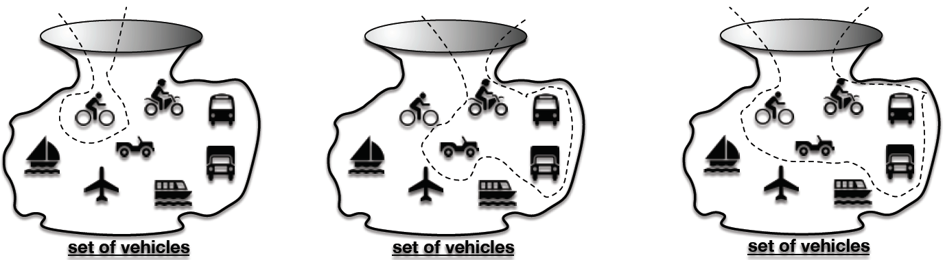
- Figure 4: Subset and union
Definitions:
Proper subset: a set that contains members that are also members of a larger set, at the same time excluding other members of the larger set. Sub-sets are, then, by definition, also a set. Union: the set of elements that belongs to either of a given pair of sets.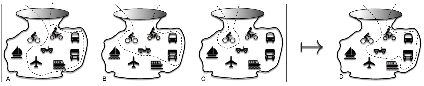
- Figure 5: Subset and difference.
- In a different way, rather than noticing a unification of two existing sets, we might start with a subset, say all of the vehicles that use energy derived from fossil fuels (i.e., airplane, motorbike, motorcar, truck, bus, boat) and want to ‘get at’ members of this set, but only those that are designed to be propelled on a road surface. This situation is presented in Figure 5. We place the vehicles that run on fossil fuels inside a bag (left-hand picture ‘A’) and we do likewise for all of the vehicles with wheels (left-hand picture ‘B’). Then we take the set of vehicles with wheels that do not use fossil fuels, the bicycle, identified previously (left-hand picture ‘C’). From these sets we can derive set ‘D’ (right-hand picture).
Definition:
Difference: the set of members of the first set that are not members of the second.- With this definition, we start with B (set of wheeled vehicles) and we ‘minus’ set A to get rid of all the vehicles that are not suitable for the road. When we have completed this operation, we minus set C from the result, the bicycle in this case, which is propelled by a human, not the burning of fossil fuel, leaving set ‘road vehicles that run on fossil fuel’, i.e., set D:
- (B - A) - C = D
- Another important aspect of set operation is where we have two separate sets, and we want to know if the two sets have any common members. The intersection provides the answer to this.
Definition:
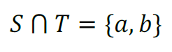
Intersection: the set of members of the first set that overlap with the second, or more generally, the set of elements that are members of two or more given sets.- An example intersection is presented in Figure 6. We have two separate sets, this time drawn inside two squares. There is the set of vehicles that pollute the atmosphere, because they burn fossil fuels in the process of acceleration, and the set of 2-wheeled vehicles. The intersection is a single member set, the motorbike, which has two wheels and pollutes. If we denote vehicles that pollute with a letter P, the set 2-wheeled vehicles with letter Q, and the single motorbike as R, then the following symbolic representation describes the same picture:
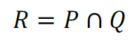
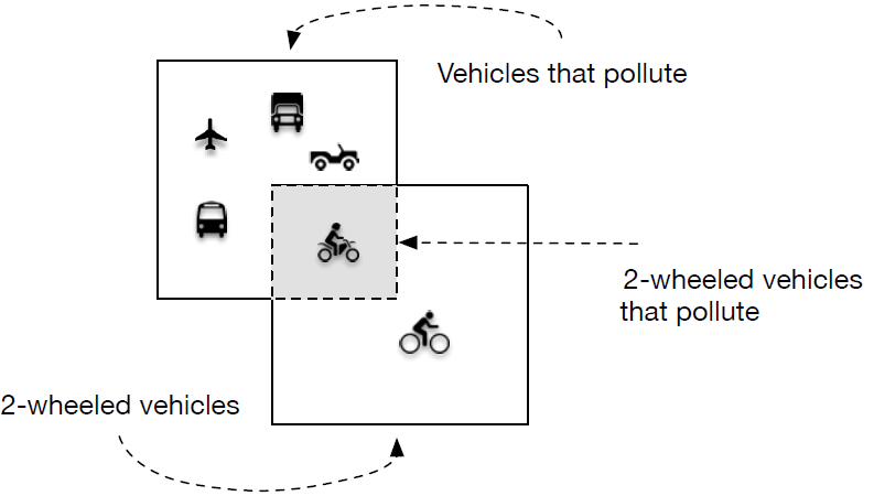
- Figure 6: Intersection of two sets.
-
3.3.2 Sets: Union, difference, intersection
- The union, difference and intersection of sets form three important operators in terms of relational databases. Up until now we have been visualising the set, and operations on sets, as two-dimensionally. Another way to do this is by using Venn diagrams.
- Venn diagrams – illustrated in Figure 7 – can be used to generally represent what is inside a given set, irrespective of what this might be. A set is represented by a circle and where there are members of sets that are the same, this is represented as the overlapping areas of the circles. We thus have three sets (A, B and C). The six example operations show different ways of identifying areas of the sets, individually, or as a combination. The shaded areas correspond to the result of the operations defined underneath the pictures. Here, we only have three sets, but the power of the set theory is that operations can be applied to any number of sets, even though this is difficult to then visualize ‘on paper’, so to speak. The different operators shown here correspond to the operation described above – i.e. ∪, ∩ ,− are the union, intersection and difference operators, respectively.
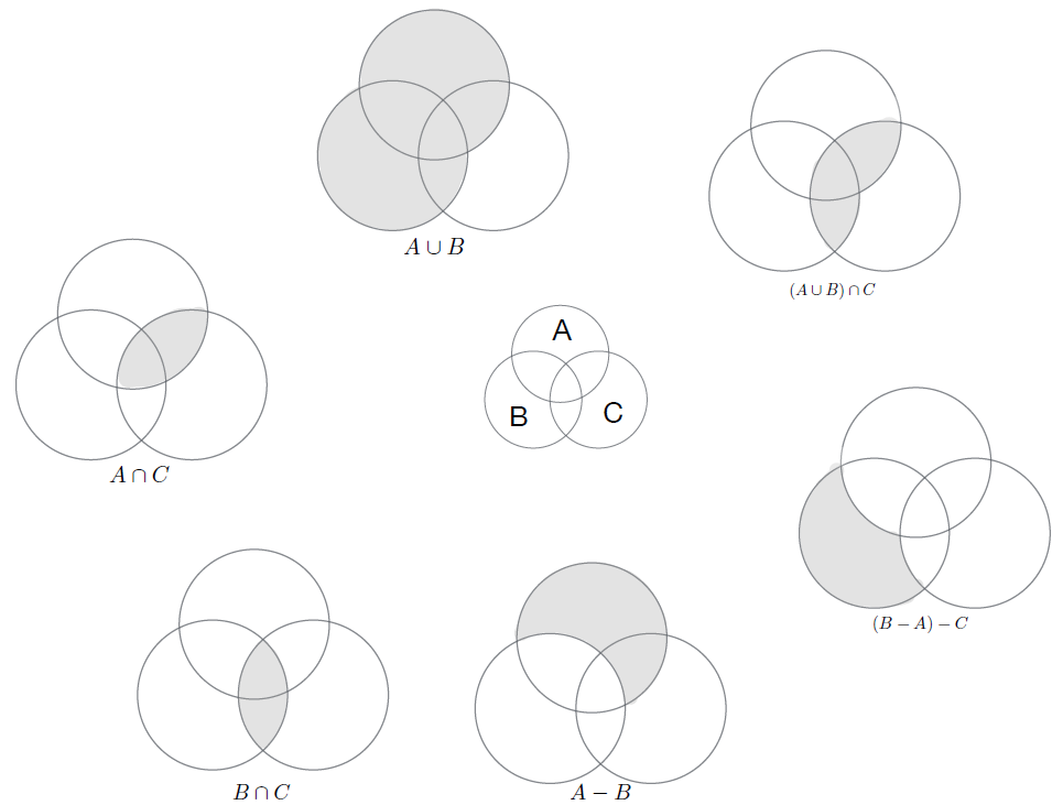
- Figure 7: Sets as Venn diagrams.
-
3.3.3 The set language relates to the query language
- You might have been wondering what all of this has to do with databases? Well, it has everything to do with them. We have previously discussed how a database is not just a way of storing a file system in memory, but is a “… shared collection of logically related data and its description, designed to meet the information needs of an organisation” (Conolly Begg 1.31). Our coverage of basic set explanations serves to highlight that sets are also logically related and this logic can be explored and exploited in the process of data modelling, such that we can access the data using, essentially, the language of set operators.
- Tip: it can be very useful to start thinking about sets, and set operations, because they underpin much of the syntax in the statements of query languages (the programming languages used to process, access and manipulate data from databases).
- We will introduce a query language known as SQL in more detail later in the course, but for now, just to demonstrate the relevance of the language of sets we present Table 1, which indicates that the typical structure of an SQL command is to SELECT a subset of data FROM a database tables (or tables), in accordance with CONDITIONS that you specify. Indeed, SELECT and FROM are SQL keywords; conditions are often usually specified with numerous other keywords (e.g., WHERE, IF etc. etc.). You are encouraged to go and research some simple SQL statements with this basic structure in mind; it will help you start to understand the logic of data selection and how databases can be ‘asked’ to give us what we want.
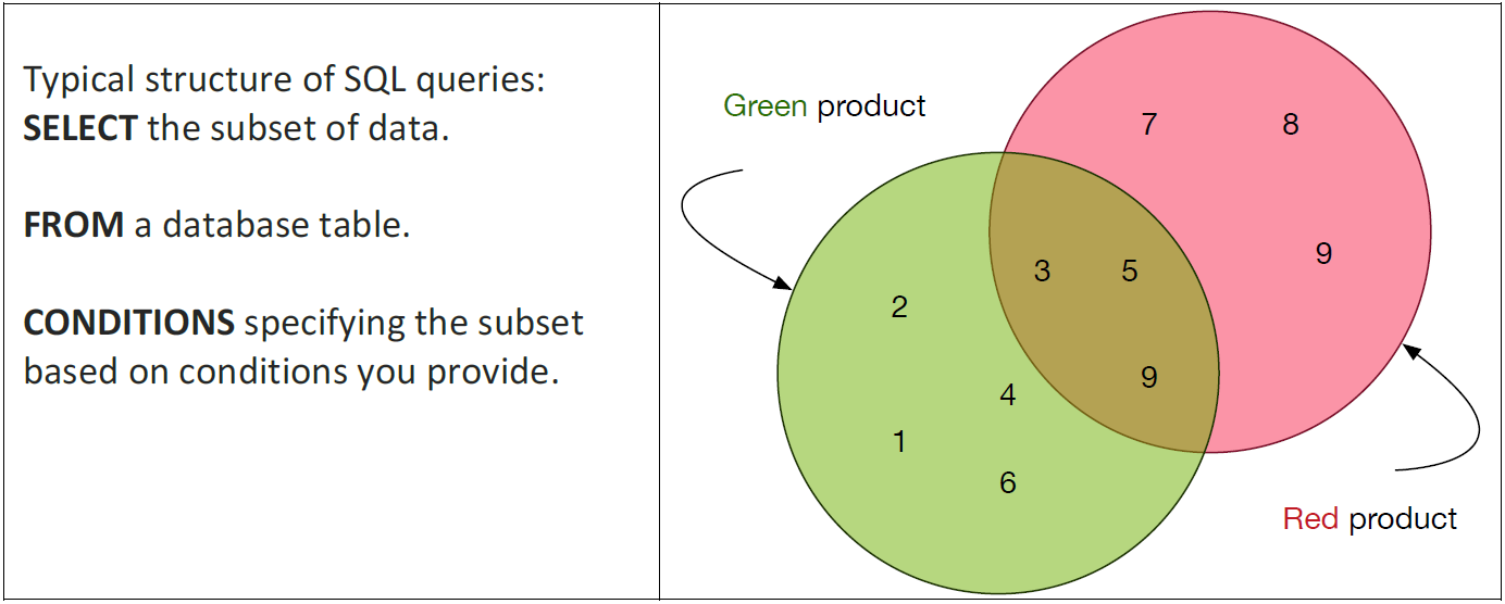
- Table 1: SQL query as Venn diagram
-
3.3.4 Relational algebra
- Relational algebra consists of a number of operations that will be useful going forwards, and so we list them here.
- Difference:
- Intersection:
- Join:
- Product:
- Project:
- Restrict:
- Union:
- You are encouraged to go and learn what these terms mean. The Ritchie book is a good place to start.
-
3.4 Summary
- ‘Modelling’ is a widely used label, in everyday life, but also heavily used within the computational sciences.
- We thus explored the meaning of models and the modelling process. This allowed us to specifically define and discuss ‘data modelling’ and ‘database modelling’ in the context of relational databases.
- Database development as a sequence of iterative steps involving conceptual modelling, logical data modelling, followed by physical data modelling.
- We introduced some standard visual diagramming techniques related to relational database modelling.
- We then introduced the language of set theory, which is the mathematical underpinning of the query language of rational databases, known as SQL.
- Download PDF Version