04
-
Relational data modelling II: from ER diagrams to the data schema
- In this week, we will cover the following topics:
- Optionality and cardinality.
- Types of relationships between different tables (one to many, many to one etc..).
- Keys: foreign keys and primary keys.
- Modelling time-dependent data.
- Physical design: data types and sequencing.
- … and will result in the following learning outcomes:
- An understanding of optionality and cardinality.
- An understanding of many-to-one, one-to-many kinds of relationships between data.
- Knowledge of how to accumulate time-relevant data into tables.
- An appreciation, from examples given, that databases are critical in the real world, e.g., for keeping freight systems in motion (and therefore our fridges stocked with food).
-
4.1 Data modelling, increasing the detail
- As previously suggested, in Week 3, during the preliminary phases of data design, there is a lot of interaction between the business client and the database designer and/or the rest of the database team. The detail of the data – i.e., the objects, attributes, relationships etc. – will be relatively vague.
- However, as the design of the database develops, the specification of these things will take on a finer resolution – specific relationships will become better defined, the attributes of objects more definitive, and, hence, the overall look of the design will become more detailed. As a consequence, the diagrams that you are likely to see in textbooks (and use in practice) will typically evolve throughout the textbook, becoming more detailed and containing additional information in them. The purpose is to allow representational the lower-level details.
- In this section we will introduce some further notation concerning the relationships between data – i.e., the optionality and cardinality of relationship(s) – using alternative notations. The purpose is to provide you with the different notations, and also visit the underlying meanings again in more detail. This will be done by considering some examples, which will again be based on the same general theme we are following: the movements of goods through a supply chain.
-
4.1.1 Optionality and cardinality
- Consider an example based on the manufacture of various products. We will call the producer of these products G&P, which is a hypothetical manufacturing company that produces various products relating to what we might classify as Home Care products…things like toothpaste, detergent, shampoo, soap, beauty cream, hairspray etc. Another company, known as Ainsburies LTD, is a separately owned retail company and it sells the products it purchases from G&P (of course it might also purchase products from other manufacturers) directly to customers through its supermarket outlets.
- We are designing a data model, for Ainsburies LTD. This is the scope of our data model. The model must handle the recording of product deliveries. A Product_Delivery entity can be thought of as relating to different products, which have the generic entity name Product. From the point of view of the Ainsuries LTD, what has to happen is that the Products need to arrive at the store. When they arrive, they will, in reality, need to be stored inside the supermarkets warehouse. However, for the purpose of our example we will not cover this storage aspect. We only cover everything up until their arrival at the store.
- To begin, we make a number of observations, with the help of the client, as follows:
- 1. Each delivery (we will refer to in-schema as Product_Delivery) will be associated with potentially many items made by G&P, but not necessarily every product (likewise, named ‘Product’ in the schema) made by G&P is part of such a delivery.
- 2. Each Product might be associated with many deliveries. This makes sense – once a store aquires a given product, the ultimate aim is to sell it and thus run the stock down, resulting in the triggering of another order, which needs to be delivered.
- 3. Each physical delivery must arrive at a given location (likewise, named ‘Location’ in the schema).
- Therefore, we have three entities (Product_Delivery, Product and Location), and, to begin with four potential relationships:
- Product_Delivery--Product.
- Product--Product_Delivery.
- Product_Delivery--Location; and
- Location--Product_Delivery.
- It is, however, helpful to define the boundaries of relationships and we would like to be more explicit about the Optionality and Cardinality of relationships, before going on to introduce a more detailed, higher-resolution database design in tabular form.
General Definitions:
Optionality: The minimum number of entities that can be associated with another entity. Cardinality: The maximum number of entities that can be associated with another entity.- Therefore, look at Table 1. We said, previously, that a Product_Delivery can contain any number of Product items, but not necessarily every product is part of a delivery. We might also realize that a delivery from G&P must contain at least one Product (a delivery which contains nothing is not a delivery of anything at all!).
- Therefore, when thinking about the relationship, Product_Delivery--Product, we say that a Product_Delivery may have 0 instance of any given Product or it may have any number of Products. Thus, the optionality is ‘0’ and the cardinality is ‘*’ (meaning “any”). On the other hand, a Product might not belong to a Product_Delivery (optionality ‘0’), but if it does, then it only belongs to a specific, singular (cardinality ‘1’) Product_Delivery. Similarly, a product delivery may not be made to a given location (optionality ‘0’), if the location is not a retail outlet, for example, but product deliveries are made to many locations (*). Finally, a Location might not receive a product delivery, (optionality ‘0’), but numerous (*) will receive deliveries.
Relationship Optionality Cardinality Product_Delivery--Product 0 * Product--Product_Delivery 0 * Product_Delivery --Location 0 * Location-- Product_Delivery 0 * - Table 1: Optionality and Cardinality
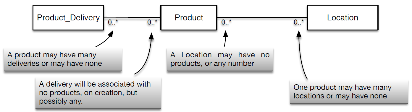
- Figure 1: Entities and Their Relationships
- Typically, the bi-directionality (the two-way property) of relationships is captured diagrammatically on a single line, to help keep diagrams neat, while at the same time allowing them to express the information required. Therefore, by way of illustration, we present a complete diagram in Figure 1. Note: the notation used here is a kind of alternative to that introduced in Week 3 (see section TDO). We do not elaborate on the differences here, but for further reference on alternative notations available, please refer to ch 3 in Ritchie (Ritchie,2002).
-
4.2 More detailed tabular diagrams of entities
- As we have suggested previously, in week 3, good databases usually follow a well-defined process of design. Due to the relatively limited scope of this document, we will follow these principles, but by focusing on a small part of what might otherwise be a much larger database design.
- In Figure 1, we introduced some simple entities and their relationships. This was in order to illustrate the ‘boundaries’ of the relationships, using a slightly different notation than previously used. We will expand on this example, here, by defining the entities more fully, which requires a tabular representation of the entities in the diagram. Through the process of the design, we end up with more entities (or even fewer) as we iterate, consequently realizing that previous choices may be unnecessarily complicated or too limited.
- Therefore, let us reconsider the boxed entities in Figure 1: Product_Delivery, Product, Location. Let us consider in a little more depth what these entities consist of in the real world, by providing natural language descriptions of them:
- Product_Delivery: physically, this can be thought of a specific trip undertaken by a vehicle of a given type, which must make the delivery (of various goods) to the store (destination) from the given location of the factory (origin). This delivery must be received within a time window – i.e., it is no good if it arrives at the store too early as there might not be enough room in the warehouse to accept the stock, but too late might result in lost sales due to lack of stock. From the point of view of a retailer, then, it is useful to monitor the performance of the supplier in this light. A time window will be defined, generally, by a start time and an end time. To distinguish the ‘expected’ time window from the ‘actual’ time window, we postfix the relevant variables with appropriate letters – ‘e’ (expected) and ‘a’ (actual). Other relevant information is the capacity of the delivery. Physically, this depends on the actual vehicle used for the delivery task. Vehicles have a maximum weight that they can carry – this is the weight beyond which adding any more weight could be dangerous and/or damage the vehicle. Similarly, if the products being shipped are quite light, then it is likely that the other capacity limitation comes into play – this is the actual volume of the truck, which cannot be exceeded for obvious reasons.
- The Product: we will keep the description of the product quite simple. Of course there are all kinds of complexities relating to a given product (branding, color, shape, etc), which do not concern us in terms of the current scope. Really, for the purpose of moving and storing a product, we need to know what kind of product it is, but then only the dimensions (weight, volume) of a given unit. Products might arrive, not as an individual item to be placed immediately on a supermarket shelf, but as a box containing several individual items and we might need to think about how we quantify the number of units etc.
- The location, indicates that the store (and the factory), might be represented by a location, rather than a full address. The reason a delivery application might have the address/location etc., stored as separate entity is because it makes sense from the point of view of easily accessing geo-coordinates for routing. Here, then, we are assuming that the company owns its own fleet of vehicles, which need to be routed, but perhaps by use of a third-party routing API that accepts a (Latitude, Longitude) geo-coordinate. Furthermore, while is important to store the postal address, Latitude, Longitude might not usually be considered as logically acceptable attributes of a postal address.
- In Figure 2, we present the corresponding design in diagrammatic form. Again, we have used yet another alternative representation for the relationships. We won’t explain these here, but we do encourage you to explore the various recommended textbooks to discover the meaning of all these different kinds of representations. The reason we have used many kinds of representation in the notes is such that you are aware that they exist, and different textbooks (and employers) will use different combinations. Try to become familiar with them all.
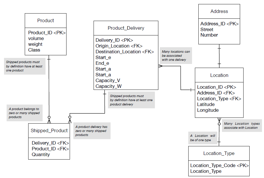
- Figure 2: Simple 'logistics' database
-
4.3 Creating tables
- In this section, we will look at some further practical steps required, which can be regarded as much closer to the process of implementing our database. In order to do this, we will concentrate not on all of the tables shown in Figure 2; data types are required to be defined in order to help databases store the appropriate values (see below)
- Let us take a look at these tables in their row/column form:
Product_ID Volume Weight Class SMALLINT FLOAT FLOAT String - Table 2: Product table in general row/column form, indicating data types.
Del..ID Ori..n Dest..n Start_e End_e Start_a End_a V_Max W_Max DATE DATE DOUBLE DOUBLE - Table 3: Product_Delivery table in row/column form, indicating more data types
- The ‘.’ Entries are there to indicate that data does exist in those cells, but we omitted them for illustrative purposes. What is important is that in order to store data inside a database, we must ‘declare’ what kind of data we are storing such that the computer can allocate the appropriate resources.
-
4.3.1 Identifying rows within a table with ‘primary keys (PK)’
- Primary keys as natural keys: We have already alluded to the use of keys. As a reminder, primary keys are special attributes of an entity in that they allow identification of specific rows. As a consequence, primary keys must be unique to a given row. Let us take our above example of a Product, made by the company G&P. We assume for ease of illustration that a ‘full’ table of products is given, assuming for now that G&P has in total a range of 8 different products.
- Primary keys:
Product_ID Volume (m^3) Weight (kg) Class 52343 10.0 20.0 DOM_CLN 29892 10.0 18.5 DOM_CLN 99892 5.0 11.0 DOM_CLN 11111 2.0 12.0 DOM_CLN 22345 1.0 8.0 PER_HYG 09234 9.0 06.8 PER_HYG 98_29 8.0 01.9 PER_HYG - Table 4: Product table in row/column form.
- Which column allows us to uniquely identify a given row. Clearly, not the Class column, which associates the product to a general product class; this is exactly the opposite of what we want. However, the Weight column has the right attributes (all of the entries are different). Nevertheless, purely from a common sense point of view, even though the Weight attribute currently has the required heterogeneity in content, it would be a poor choice for a primary key; this is because, given the development of new products, there would be a risk of the weight getting duplicated, especially if only the fragrance of an existing cleaning product were changed to differentiate a ‘new product’. Therefore, from the existing columns, the best choice to use is the Product_ID column. The column contains a set of entries, none of which are duplicates.
- The main thing to remember about keys is that the identify a given row. However, as suggested, some common sense needs to be applied when choosing primary key. We employ the phrase common sense loosely – this sense might not necessarily be obvious given a set of data taken at face value. This is why, again, it is important for the database development team to work closely with the client in question and get to learn the various data owned by the company, how it is used, to think about the data types, the implications this has for use as a key etc.
- Primary keys as composite keys: Sometimes the structure of a table may not allow the identification of a primary key. One choice is simply to generate a key (see below, Primary key as synthetic key), artificially. However, if we want to persist with the using the actual data, we might need to introduce more columns, and reach a point where the concatenation of columns results in a unique identifier In this way, it possibly to concatenate a number of; Ritchie (2002) contains a more complicated example involving three attributes/columns concatenated to act as a single primary key (Ritchie, 2002, p 27). It is useful to understand this more complicated construction of primary keys – in practice, as a database developer, you will certainly come across them.
- Primary keys as synthetic keys: Often, natural keys cannot be found. In this case, another choice is the generate an additional attribute (often an integer) to uniquely identify a row. One way to guarantee uniqueness is to use an integer, for example, that is incremented each time a row is added to the data table. Consequently, each subsequent row will have an identifying attribute that is unique. This is a common way in which to define primary keys.
Summary of some key definitions:
Natural key: an attribute in the data, which can be used to uniquely identify a row. Composite key: attributes in the data, which when concatenated, can be used to uniquely identify a row. Synthetic: a key that is generated purely for the purpose of uniquely identifying a row. -
4.4 Creating relationships between tables
4.4.1 Many-to-many example
- Consider the following example about the delivery of products from a given manufacturer to a destination retail store. Goods, physically, will be loaded onto a vehicle that has a maximum weight and volume (capacity). The vehicle will be expected at the store at a given time, although the actual time will need to be recorded; these features are captured by the <Product_Delivery> table whose Delivery_ID is a generated integer and primary key. The <Product> is described as above, again, with a generated integer, <Product_ID>, and the primary key. Importantly, for a many-to-many relationship a link-table must be created. Please see Table 4 The link table allows many products to be associated with products deliveries and many product deliveries to be associated with products.
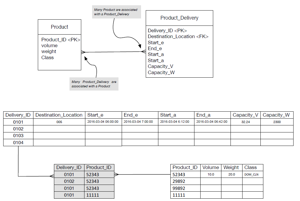
- Figure 3: Many to many example with link-table
-
4.4.2 One to many example rows in other tables with foreign keys
- We have used the example in Figure 3 to demonstrate a many-to-many relationship (numerous other examples can be found in the recommended textbooks for the course). However, while the use of a link table is the method to achieve the many-to-many relationship between entities, generally, we will take a closer look at the example given and have a think about what other data might be useful to capture (something, perhaps that the client did not tell us, explicitly, but that we noticed would be a useful to introduce into the data schema)…
- Currently, the design in Figure 3 assumes that each product is loaded individually to the truck, in whatever unit this means in the application domain (a case, a pallet etc.). This unit is associated with the appropriate weight and volume. However, would it not be useful to capture the quantity of units placed into the vehicle?
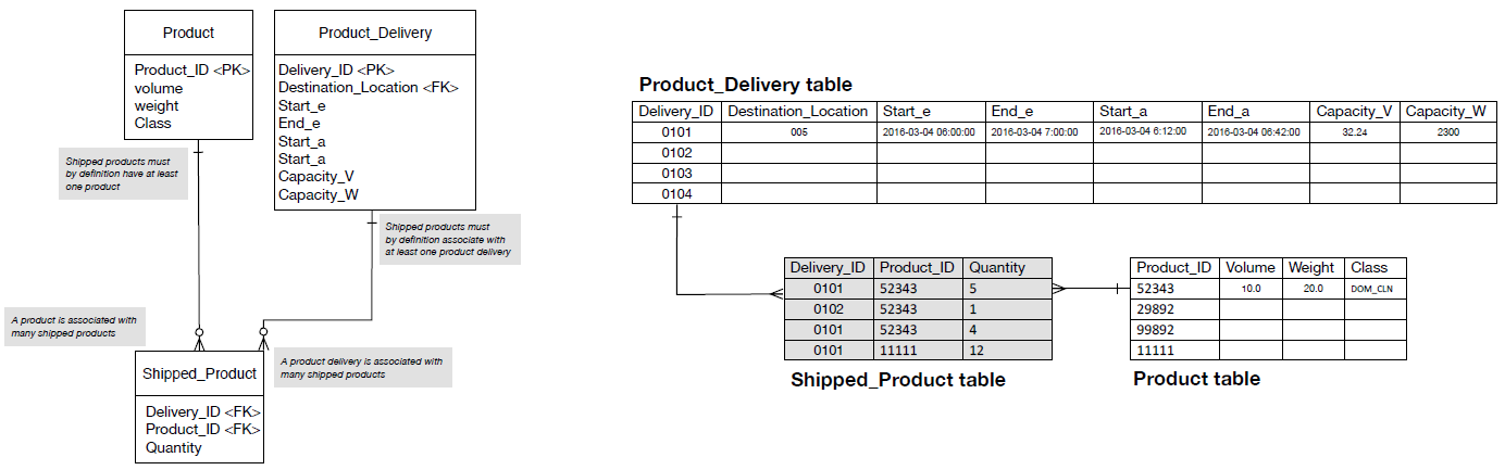
- Figure 4: One to many relationships
- The quantity of units is not a natural attribute of <Product>, and we want to keep the <Product_Delivery> entity clean from such details as well. One choice, therefore, might be to introduce a new entity called <Shipped_Product>, which will perform a similar function as the above, many-to-many relationships, shown in Figure 3, but also contain the <Quantity> of units.
- This scenario is presented in Figure 4. The new design contains foreign keys to the <Product> and <Product_Delivery> entities. Notice, also that the many-to-many relationship between <Product_Delivery> and <Product> has disappeared…or has it? Actually, this relationship can still be thought of as existing, but now it exists through the new entity <Shipped_Product>. Therefore, the introduction of this new entity allows us to maintain some of the previous logic, but at the same time make the data more useful. For example, if we want to know the quantity of products shipped (by weight, volume, product type, unit quantity etc.), we will be able to derive this information by executing the appropriate queries of the database.
-
4.4.3 Modelling time-dependent data in tables
- An often-important characteristic of products is of course their price. This is not captured in the above example, so let us consider a different logistics context to the one presented...
- Let us imagine that freight companies are increasingly under pressure to monitor their costs, and their GHG emissions. This can be done in several ways, but let us assume an ‘internet of things’ application. It is well-known, which we take as given, within in the freight sector that driver behavior can affect the uptake of fuel. For example, large accelerations can result in the burning of additional fuel, increasing costs and GHG emissions. Therefore, a device has been created by ‘ANP’, an analytics company, to sit on-board vehicles and monitor accelerations. Data is streamed to a remote server stored in a database, which also belongs to an Analytics company ‘ANP’. Freight companies (e.g., ‘G&P’ and ‘Marks’) outsource analysis to ‘ANP’.
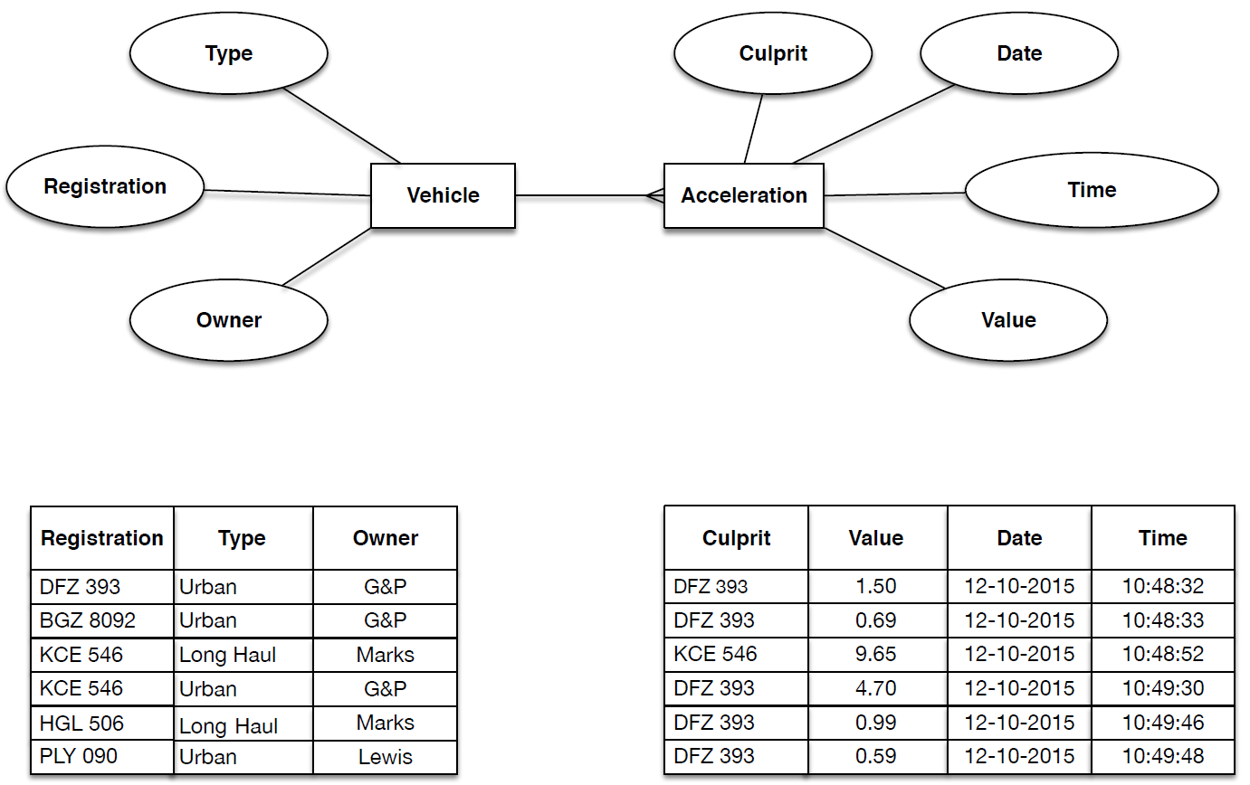
- Figure 5: Database model for vehicle accelerations
- How might ‘ANP’ represent this data as a database? An example is provided in Figure 5. Notice the relationship here: Vehicle may have many Accelerations. We might imagine a situation where, once an acceleration goes above some threshold, it is reported to the database (as in the example provided), such that time sampling is non-uniform in frequency. This is relevant to the current situation, where the two companies are interested in identifying drivers who over-accelerate, such that training can then be provided. We might however, just as easily imagine a situation where the accelerations are required at even frequencies in time, regardless of the values. This is often the requirement in the field of time series analysis.
- Again, this situation concerning the dynamic capture of data is achieved using a table, where each row enters a value for the specific time, here per-vehicle-acceleration. This is a common technique for time dependent data modelling, as other examples in the literature demonstrate (e.g., see Ritchie ch 4).
-
4.5 Physical Design
4.5.1 Data types
- This is an important part of defining the database in more detail, and it is important to recognize that datatypes in a database have a slightly different usage compared with those in a programming language such as Java. As Allardice states:
- “Database systems want you to be much more specific about your columns than a programming language wants you to be about your variables.. so that they can be efficient about storing and indexing them, and so it can enforce your rules”.
- Allardice (2015)
Some database data types (MySql)
Numeric:
INT, TINYINT, SMALLINT, MEDIUMINT, BIGINT, FLOAT, DOUBLE (DECIMAL), REAL (NUMERIC).
Date and Time:
DATE, DATETIME, TIMESTAMP, TIME, YEAR.
String:
CHAR, VARCHAR, BLOB (TEXT), TINYBLOB (TINYTEXT), MEDIUMBLOB (MEDIUMTEXT), LONGBLOB (LONGTEXT), ENUM.- In other words, the data types in database systems have a wider range of options. We will not go through all of the data types here. However, let us look at the example of integer data types in MySql, as presented in Figure 6.
Type Storage Minimum Value Maximum Value (Bytes) (Signed/Unsigned) (Signed/Unsigned) TINYINT 1 -128 127 0 255 SMALLINT 2 -32768 32767 0 65535 MEDIUMINT 3 -8388608 8388607 0 16777215 INT 4 -2147483648 2147483647 0 4294967295 BIGINT 8 -9223372036854775808 9223372036854775807 0 18446744073709551615 - Figure 6: Integer data types in MySql.
- In Java, native integer types (short, int, long) are stored in chunks of memory known as bytes. A short typed variable uses up 2 bytes, an int 4 bytes, and a long 8 bytes. Compare this with the integer choices in MySql. Here, we can choose intermediate numbers of bytes (3 for MEDIUMINT) and only one byte (TINYINT). When you are developing a Java application, it is not always necessary to optimize the use of memory, and developers of such applications are, generally, more relaxed about these issues (this does not mean that it is not sometimes important). On the other hand, databases are often designed and used to store data, which accumulates over time. It can, therefore, become much more important to think about the usage of memory and the potential space of memory required for certain attributes ahead of time. Essentially, the additional options of the types, as illustrated in the above figure for MySql, allow the programmer more control over the use of computational resources.
-
4.5.2 Identity using automatic sequencing
- Elsewhere, we has discussed the use of keys to access rows of data in a unique way, and some different ways in which this can be achieved. SQL databases support the automatic generation of identity columns. These columns typically take the form of mathematical sequence. A sequence is an ordered set of natural numbers/integers. As such, each number in sequence is guaranteed to be unique and therefore an excellent choice to use to uniquely access any given row in a database table.
- Let us look at some MySQL code. You can follow the comments to see the meaning of the code. However, of most relevance here is the creation of the ‘ID’ attribute (first emboldened line). The NOT NULL AUTO_INCREMENT means that the ID value cannot be null and will be automatically incremented by 1, each time a row is added to the database. The Name entity must also have a value, but the ID is set as the primary key.
- So, running the following code will result in a table named People that sits inside the Populations database.
# This is very straightforward to create a database Populations CREATE DATABASE Populations; # Create a table named People inside the Populations database # CREATE TABLE Populations.People ( ID int NOT NULL AUTO_INCREMENT, Name varchar(255) NOT NULL, PRIMARY KEY (ID) ); # Load the names John, Jeff, Sarah, James into the People table # that now exists in the Populations database # INSERT INTO Populations.People (name) VALUES('John'),('Jeff'),('Sarah'),('James');- Then, running the following command:
SELECT * FROM Populations.People;
- …we get the output:
ID Name 1
2
3
4John
Jeff
Sarah
James- …where we can see that the ID has been automatically generated with incremented values, alongside the name values added manually by the above code.
-
4.5.3 Indexing
- This is a useful point and which we can consider the topic of ‘indexing’. In this context, it is important to realise, taking the above output as an example, that the visible ordering of a table, when viewed, is not necessarily representative of the way that the data is stored on disk.
- Therefore, if you want to find a given row, it is very useful from a ‘computational speed’ point of view to order the data in a meaningful way, that is from the point of view of the machine that needs to retrieve the data. To speed up the processing of data, we use indexing.
- In most database management systems indexing is implicitly implemented on the primary key. For example, in the People table we created above, if we wanted to access ‘Sarah’, and we did this using the primary key we would execute in MySQL the following:
select Name from Populations.People WHERE ID = 3;
- then the computer would know exactly where to look and return the required information in optimal time. This is because, ‘ID’ is the primary key and therefore what is known as the ‘clustered index’. The machine can therefore jump straight to the required address to get the data.
- However, we might find ourselves writing alternative queries. For example, if we wanted to access Sarah by name:
select Name from Populations.People WHERE Name = 'Sarah';
- In this case, the computational search process will not rely on efficient indexing. Imagine that, to access ‘Sarah’, we first start with a name at the top of the table then read down the table reading each Name value (John, Jeff) in turn, before reaching and finding ‘Sarah’. This is an extremely inefficient way to find data and queries that result in this kind of search will take a long time to execute in large tables. Obviously, in the very simple table we considered, ‘Sarah’ is only on the third row; finding this will not take long. Alternatively, and more realistically, imagine that we have a table with hundreds of thousands of names in it!!
- While the clustered index is reserve the primary key, it is possible to create non-clustered index on non-primary key attributes. For example, we can create a non-clustered index on the Name attribute.
- A number of points are worth summarizing regarding indexing:
- Indexes allow computers to search efficiently for the data required from a database.
- The primary key is usually the ‘clustered’ index, which is a kind of default index that allows efficient primary key based querying.
- Non-clustered indices can be created where queries are often done without primary keys.
- There are trade-offs associated with indexing. Nothing comes for free when you use a computer. Creating index, for example, requires the use of memory and increases database maintenance, even there the trade-off is increased processing of queries.
-
4.6 Summary
- We learnt more details of entity relationship modelling.
- Continuing with a ‘logistics’ example we arrived at a simple design for a logistics database.
- We then moved on to some of the practical issues regarding the creation of tables, e.g., specific datatypes must be explicitly declared when creating tables. We highlighted some of the datatypes available in the MySQL implementation of SQL.
- We then discussed primary keys and synthetic keys before returning to the issue of creating relationships between tables, using link-tables, to specify different kinds of relationships between tables/entities.
- Download PDF Version