05
-
Normalising relational data
- In this week, we will cover the following topics:
- Anomalies that can occur when modifying a database.
- The process of data optimisation (a.k.a data normalisation).
- Basic data normalisation steps, 0NF, 1NF, 2NF, 3NF.
- An example of data normalisation, from first to third normal form.
- … and will result in the following learning outcomes:
- An understanding of some different kinds of anomalies, and therefore why structuring data in a specific way to help avoid these anomalies is important.
- An understanding of normalisation as a sequential process.
- A practical knowledge of what to do when normalising a relational database.
-
5.1 Overview
- The process of normalization is a way of ensuring that the structure of your database is welldesigned. In this context, well-designed means from the point of view of:
- data storage and;
- data integrity.
- To improve memory usage and data integrity, it is important that the data is stored just once inside a database. Of course, the reason that this is a good thing from the point of view of memory is very obvious. From the point of view of data integrity, and we have touched on this previously, it is advantageous wherever possible to store a single copy of any given datum. Example important reasons are that if a datum is stored more than once, then:
- each separate storage location needs to be updated, whenever there is a change in the data itself.
- each separate storage may result in more search, whenever there is a query concerning the datum.
- alterations to the data must be kept consistent if the database is to remain useful, otherwise, the thought-of single datum, in fact, becomes fragmented into erroneous copies of itself. This can lead to major problems.
- each separate storage takes up additional memory, resulting in redundancy and increased cost.
- Normalisation is:
“A formal procedure … that can be followed to organise data into a standard format which avoids many processing difficulties.”
Ritchie (2002)
a procedure to produce data with “the minimal number of attributes to support the data requirements of the enterprise; attributes with a close logical relationship …[placed] in the same relation; minimal redundancy, with each attribute represented only once…with the exception of foreign keys”.
Connolly and Begg (2015)
“not an ivory tower, theoretical, academic thing that people talk about but no-body really does in the real-world. No. Everybody does this. If you are a working database administrator or database designer you can do normalization in your sleep. It is a core competency of the job.”
Allardice (2015)- Therefore, normalization is important because it is a highly pragmatic way of guiding you through some steps to improve your database.
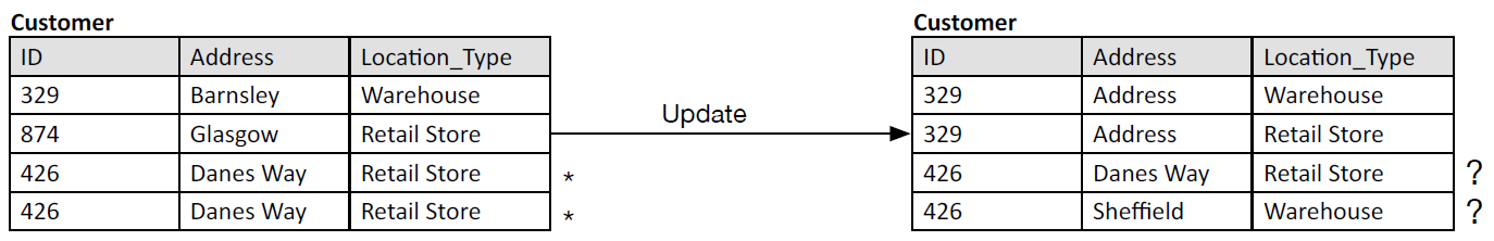
- Figure 1: Update anomaly.
-
5.2 The problem of data modification anomalies
- In relational database design, the normalization process should prevent the occurrence of modification anomalies. It is impossible to cover all of the possible examples of anomalies, and you will come across many different examples in the literature, but in order to give you an idea of what modification anomalies are, we present one example for each modification anomaly type, as follows: update anomaly, insertion anomaly, deletion anomaly.
-
5.2.1 Example: update anomaly
- Consider a situation where a manufacturer, of computers say, distributes computers to various Customers. Please see Figure 1. Within its database the customer table includes, among other things, the following: a customer ID, a customer address and the type of building at that address. Unfortunately, in this case, the table is poorly populated. Firstly, the Customer with ID = 426 has two entries for the address, by mistake. In and of itself this duplication is a waste of memory.
- However, now for the more serious more serious problem… The customer, quite a large company, has always taken computer orders from the manufacturer to be delivered to its warehouse. However, a change in supply chain strategy meant that the company now orders computers directly to the retail store, discontinuing the orders to the Warehouse. In this case, the duplication is more serious. The update is made, but unfortunately only to one of the entries for Customer with ID = 426, causing an anomaly; customer ID 426 is not a key for two different addresses!! As a consequence, a very simple query to find the address of Customer 426 is problematic, because the data is inconsistent.
-
5.2.2 Example: insertion anomaly
- Consider a situation where an online retailer, allows customers to register an online account. Please see Figure 2. In the database, it must be possible to store this information independently of any purchases. Therefore, another example of a poor design would be a table that did not respect this requirement and, for example, coupled the data concerning the customer details with the details of purchased product. For those customers who purchased a product at the time of registration, this would be unproblematic, but for the customer who registers with the intention to return to the website and purchase a product there are no products currently associated with them.
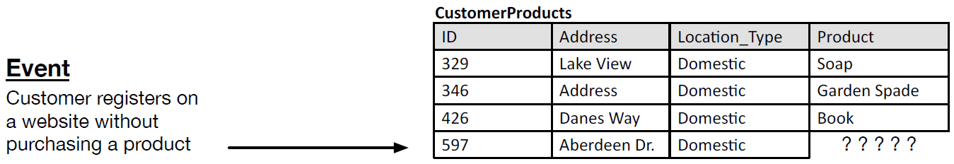
- Figure 2: Insertion anomaly.
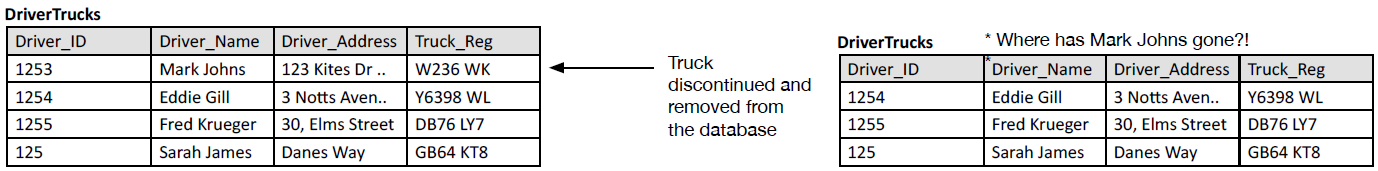
- Figure 3: Deletion anomaly.
-
5.2.3 Example: deletion anomaly
- Consider a situation where a logistics company holds a set of drivers in a database within a table where the trucks associated with the drivers are also kept. Please see Figure 3. Again, this is a situation where the data is tightly coupled. For example, after a truck has travelled a certain mileage, the company has a policy of discontinuing its service (sending it to the scrap yard). Consequently, there is no need for the truck registration to remain in the database. However, as we delete the truck from this data, we also delete the associated driver because the driver information is stored in the same table, and Mark Johns can only drive this specific truck due to the compatibility of his driving licence with other trucks in the fleet. Of course, this is a problem with the database – when we get rid of the truck we do not in the real world also get rid of the driver from the company. This is a deletion anomaly.
-
5.3 The process of data optimisation
- The process of normalisation is exactly that, a process, number of steps, a kind of recipe for baking a well-designed database. In this course we will concentrate on the first three steps of the process, which in fact goes up to seven steps in total. However, do not be concerned that you will be ‘missing’ 4 steps; the first three steps are often sufficient to produce a working database system with a high degree of internal consistency. Normalisation is often thought of as a process of optimisation, in the sense that minimises the memory needed to store data and minimises the exposure of the database to errors of input on the part of a user.
- It is important to realise that the process of normalisation follows a number of sequential steps. That is, in order to get to the second step, you must have ensured that your database conforms to the required output of the previous step, and in order to get to the next step you must also therefore complete the current step. From an un-normalised database, where we begin the process, there are three steps required to get to the third normal form, our required destination for this week:
- Begin with your un-normalised database (UNF).
- This database will typically have tables, where primary keys etc. might have been identified, but where the tables contain repeated groups, e.g. attributes that have been duplicated or even appear as groups of what should otherwise be attributes, but are contained within cells as something akin to arrays (this is simply not allowed).
- Step 1: Repeating groups must be identified and removed from the database. This is done such that each repeated group maps to a single attribute within entity/table. This will typically involve the creation of additional tables. After this step is successfully completed your database is in first normal form (1NF).
- Each of your columns represents a single attribute, which is therefore not repeated in any other column, and the normalised table contains one value per cell.
- Step 2: Make sure that your database is in first normal form before you begin. Then make sure that each non-key field depends on the entire primary key. Otherwise, rearrange your database to ensure that fields not dependent on all parts of the primary key are arranged into a table such they then depend on the entire primary key. After this step is successfully completed your database is in second normal form (2NF).
- Now, each of your fields depends on the entire primary key of the table they are in. Note, if you are not using composite keys this is no problem, you can just go to the next step.
- Step 3: We need to identify whether or not any of the non-key fields are dependent on any of the other non-key fields. If they are, then these dependencies need to be represented in separate tables such that the dependent field has as its key the field it depends on. After this step is successfully completed your database is in third normal form (3NF).
- Now, there are no non-key fields that are dependent on other non-key fields.
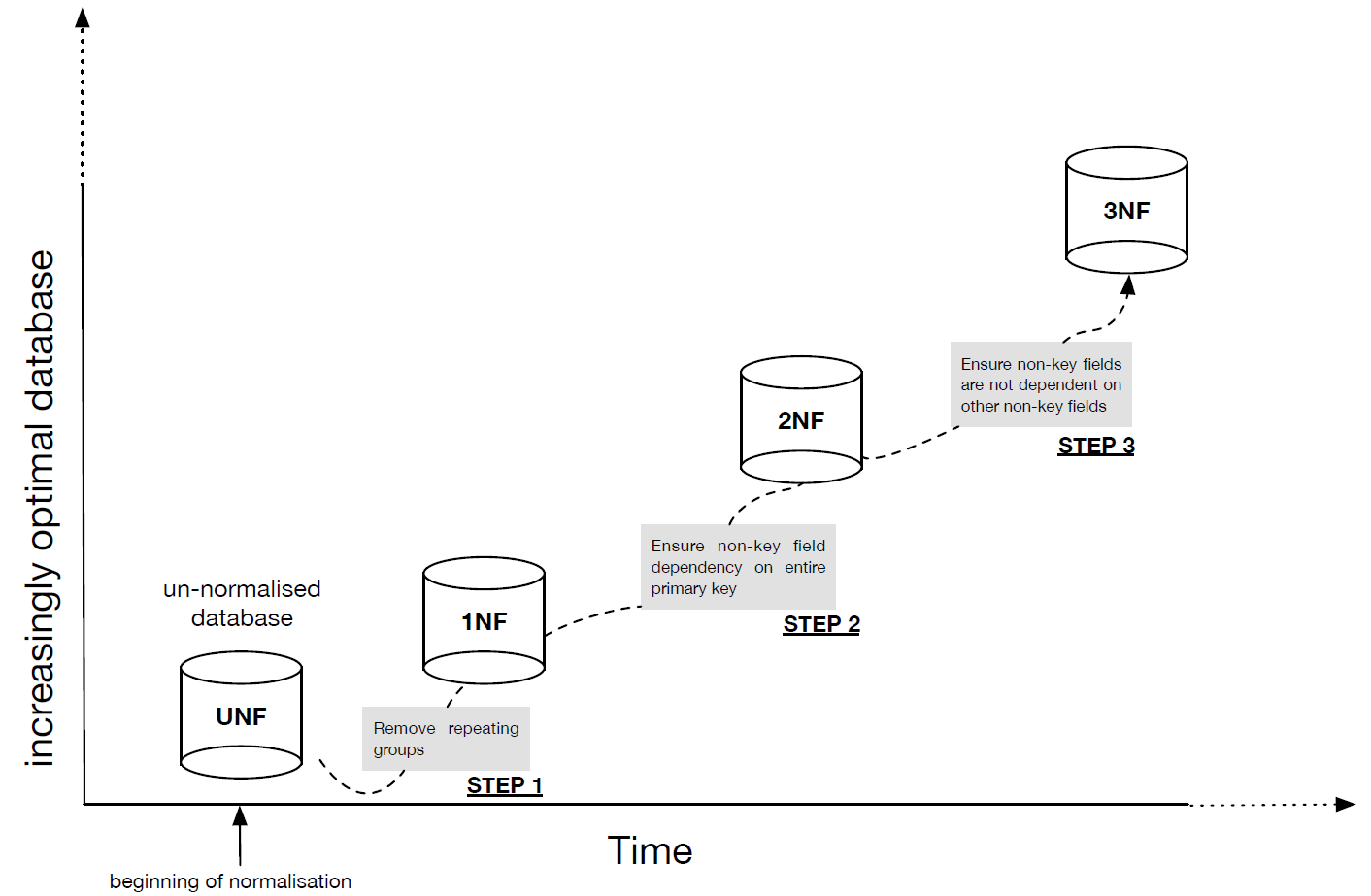
- Figure 4: Sequential process of normalization.
- Note: do not worry, if you do not yet fully understand these steps as they are written here (or indeed in textbooks). The process of normalisation is an involved practical process, and we will provide some examples below that relate back to the above descriptions. The intention will be to provide you with a single, but fairly realistic, practical example, which once you understand you can then use as a basis to understand other examples in the various literature. Before we do this, we will cover the idea of functional dependency.
-
5.4 The ruling part & functional dependency
- During the process of normalisation, it is common that functional dependencies should be identified during the construction of new tables, to de-couple data, which could otherwise more easily result in anomalies such as those given as examples, above. In order to appreciate what a functional dependency is, (in the example scenarios given below we will identify functional dependencies concerning an invoice example) we first introduce a little more set notation, with an example given already.
-
5.4.1 Product set and relation
- In Week 3 we covered some ideas behind sets, which allowed us to think of data as part of a set as a full set in itself. Here, we also need to cover a little more about sets (just notation, really, rather than any theory) in order that we can clearly understand the idea of functional dependency, which is based on the idea of relations (these are not relationships).
- A set can be defined by enclosing the members inside the following brackets {}. Consider a set of numbers, i.e., Driver_ID = X:
X_ID = {1253, 1254, 1255, 125}- And a set of strings, Truck_Reg = Y:
Y_Reg = {W236WK, Y6398WL, DB76LY7, GB64KT8}- The ‘product set’ is the set of ordered pairs, denoted X.Y:
X.Y = {1253 W236WK, 1253 Y6398WL, 1253 DB76LY7, 1253 GB64KT8, 1254 W236WK, 1254 Y6398WL, 1254 DB76LY7, 1254 GB64KT8, 1255 W236WK, 1255 Y6398WL, 1255 DB76LY7, 1255 GB64KT8, 125 W236WK, 125 Y6398WL, 125 DB76LY7, 125 GB64KT8}- …and a relation R(X, Y):
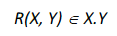
- … is a subset of the product set. There is no mystery to any of this and the same information given, here, can be drawn inside a diagram. In Figure 5 we, therefore, draw the product set X.Y and a number of example relations.
- Figure 5: Product set and example sub-sets ('relations')
-
5.4.2 Functional dependency
- An obvious pattern seen in Figure 5 is that all of the arrows are pointing from the X (Driver_Id) set to the Y(Truck_Reg). This is to represent functional dependency.
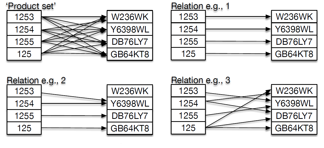
- Figure 6: Functional dependency
Definitions:
Relation: A set of ordered pairs whose order exhibits functional dependency between the ruling part (aka., primary key) and the dependent part. Functional dependency: where each value in a given set Y is associated with exactly one value in another set X, then Y is said to be functionally dependent on X.- Note. In the above examples we have used data that has already been ‘designed’ to contain a ruling part, in order to help us with the definitions given. However, it is important to realise that in a real-word situation, it is not always desirable to generate primary keys because they take up computational resources (memory). Therefore, it is common that the data is analysed to uncover any potential natural keys (parts of the data that act like X, as described above). A discussion of this can be found in the recommended textbook (Connolly and Begg, 2015) – see Chapter 14, section 14.4). This will give you a better idea of the process that occurs in practice in order to identify functional dependencies.
-
5.5 Normalisation scenario: the invoice
- Our scenario is straightforward. The company G&P Ltd has delivered a batch of products to a company (who are therefore a customer of G&P, and they are known as ‘Test Customer’). Our job in this section is to identify a database design by starting with some data from a company (an invoice), then using normalisation to produce a set of well-defined tables and relations. This process is therefore slightly different to the one implied by the previous weeks, where we have looked at top-down processes of design by using entity relationship diagrams, first, as a route to producing our final-form tables. Normalisation can be used during a process of bottom-up design where we directly apply the normalisation steps to the client data.
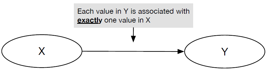
- The invoice we have to hand is presented in Figure 7. We will be looking at the problem from the perspective of G & P Ltd. It is their database that we will be creating. Take a look at the invoice, from the point of view of G & P Ltd and have a think about the important data. For example, is the address of G & P important to include in the database? The date? The invoice number? the customer name and customer reference number etc.? These are all questions you need to ask right in the beginning.
- Figure 7: Invoice data scenario
- In this example we will work on the following assumptions. The following data is important from the point of view of G & P Ltd and, for ease of drawing diagrams we decide that we will have a short-hand identifier (the name to be used within the database) for each piece of relevant data. The following table (not in the sense of entities and relationships) is produced, which is just a list of the relevant data and a description/justification, followed by the identifier:
Data Description/Justification Identifier Invoice number A recording of the invoice itself. Inv_No Customer name The name of the customer Cust_Name Customer number Unique identity of the customer. Cust_No Customer address The address of the customer Cust_Adr Invoice date The date on which the invoice was printed. Inv_Date Product_ID The unique identity of a product. Product_ID Product description A written description of the product to help a human easily identify the product. Description Unit_Price The price per single unit of the product. Unit_Price Quantity The quantity of units bought by the customer. Quantity Price The Unit_Price multipled by the Quantity. Price Total Sum of prices Total - Notice that when you are designing a database, and you have client data to hand, there might well be data that is available but which you want to ignore. For example, in this case we are interested in representing the invoice itself, and any other relevant information, but not to the point where we also including information about the ‘Payment options’ (bottom of invoice) because, for this example, we only want to capture the invoice data, which is logically distinct from exactly how (Visa, Cheque, BACS payment etc) the client might pay.
-
5.5.1 Creating first normal form (1NF)
- We have identified the data we are dealing with. We are now ready to move from this data to 1NF. Firstly, however, let us take a look at the list of data, above, when all of the data is included, including all of the repeated data, as a table we might recognise better as an entity table called Invoice. This table is presented in Figure 8.
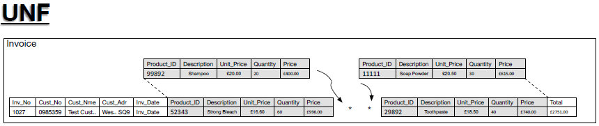
- Figure 8: Invoice as an table/entity
- The un-normalised form of the invoice as a table includes all of the repeated patters in the data. That is all of the repeated entries for the items bough by the company.
- So, the processes of normalisation states that to reach 1NF, from UNF, we need to:
- REMOVE ALL REPEATING GROUPS OF DATA
- Repeating groups are placed into their own table.
- In this example, the repetition is apparent as repeating groups (*) of a set of attributes in the invoice table, which we will call ‘Product Detail’ = {Product_ID, Description, Unit_Price, Quantity, Price}. These groups and the data are highlighted in grey, in Figure 8, the groups that need to be placed into their own table. The 1NF form of the invoice database is now presented in Figure 9.
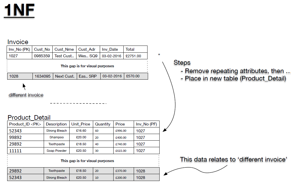
- Figure 9: Invoice database (1NF)
-
5.5.2 Second normal form (2NF)
- The second normal form (2NF) requires that non-key fields are dependent on the entire primary key. In the example we are using, the Invoice table is fine from this point of view. All non-key fields depend on the primary key by definition of the primary key (i.e., the primary key is a not a composite key) However, let us take a look at the Product_Detail table more closely. If we only use the Product_ID as the primary key there is a problem because the Product_ID field can repeat across different invoices. This is true in the example where the ‘different invoice’ (invoice number 1028) data overlaps products that exist in association with the existing invoice data (invoice number 1027).
- However, given that in each separate invoice we record the quantity of products purchased with the same Product_ID, then we expect that the Product_ID is unique to each individual invoice, and thus each invoice number. As a consequence, we can combine the invoice number Inv_No with the Product_ID to produce a composite key, which is then also the primary key. We have re-arranged the Product_Detail table. Take a look at this table and convince yourself that this is the case, that the composite key is unique.
Product_ID Inv_No Description Unit_Price Quantity Price 52343 1027 Strong Bleach £16.60 60 £996 99892 1027 Shampoo £20.00 20 £400 29892 1027 Toothpaste £18.50 40 £740 11111 1027 Soap Powder £20.50 30 £615 29892 1028 Toothpaste £18.50 20 £370 52343 1028 Strong Bleach £20.50 10 £200 - Table 1: Product_Detail.
- Now, remember, 2NF applies to composite keys. So for this example we now ask ourselves the relevant question:
- Are there any non-key fields (cells in white) that are not dependent on the entire primary key?
- The answer is yes. For example, the Description fields and the Unit_Price fields depend only on the Product_Id. That is, if we alter the invoice number, these values remain the same, but the values do vary depending on what that product is (identified with the Product_Id). As a consequence, we separate the data into appropriate tables. In this case we move the Quantity and Price into a new table called Invoice_Detail, maintaining the composite key to link this detail to the invoice in question and the appropriate products, both as foreign keys. Remaining in the Product_Detail table are only those fields that relate to the Product_Id, keeping the association with the invoice in question as a foreign key. The new tables, presented in Figure 10, are in second normal form (2NF).
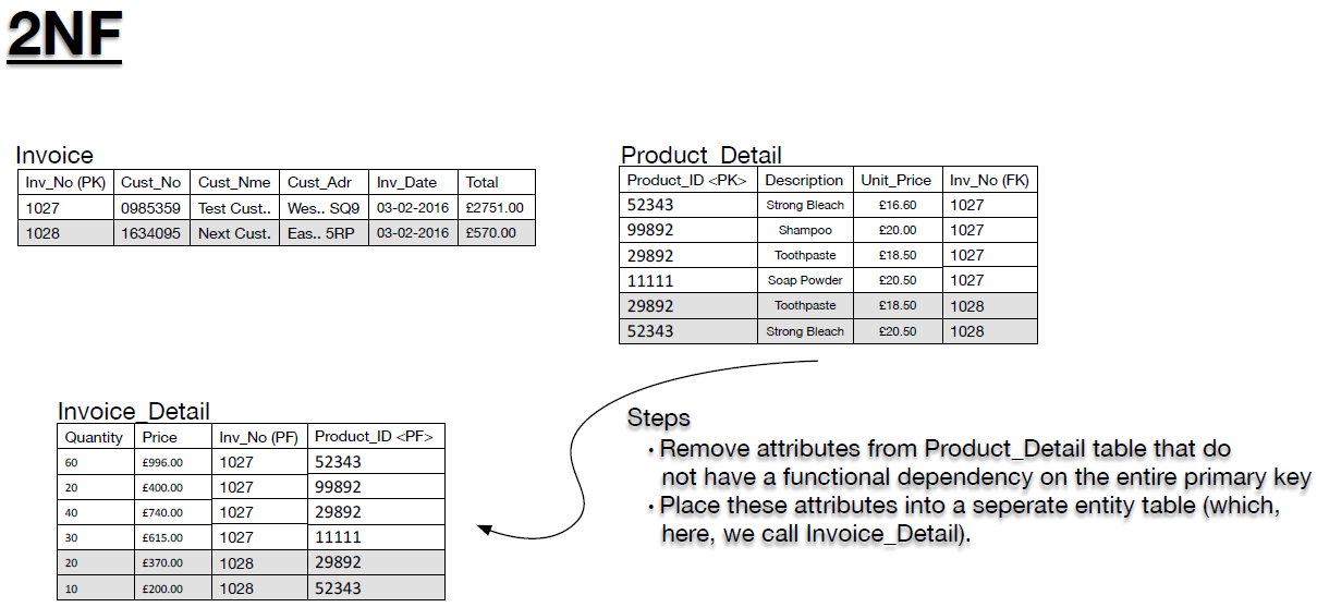
- Figure 10: Invoice database (2NF)
-
5.5.3 Third normal form (3NF)
- In order to arrive at 3NF we need to look again at all of the tables and ask:
- are any of the non-key fields are dependent on any of the other non-key fields?
- Again, an example helps. If we look again at Figure 10, then we can see that the customer address (Cust_Adr) and the customer name (Cust_Nme) are, really, dependent on the customer number (Cust_No). They are dependent in a technical sense on the invoice number, but the idea is to move clearly defined dependencies into separate tales. Therefore, we might rephrase the question we ask to arrive at 3NF:
- Are there any key fields that are acting as the key for non-key fields, but look as though they shouldn’t be.
- If the answer to either of the above questions is yes, then the identified dependencies need to be represented in separate tables such that the dependent field has as its key the field that it should depends on. After this step is successfully completed your database is in third normal form (3NF). Following our example, we present this final step in Figure 11.
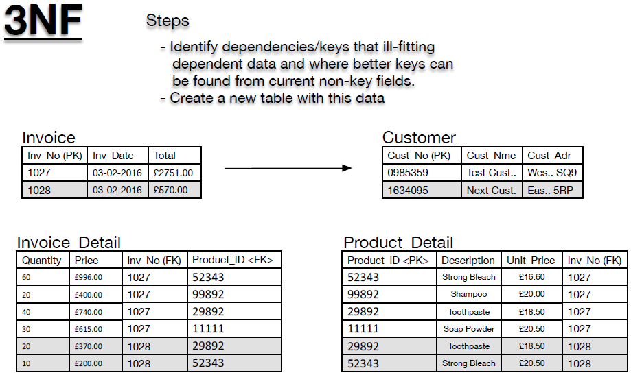
- Figure 11: Invoice database (3NF)
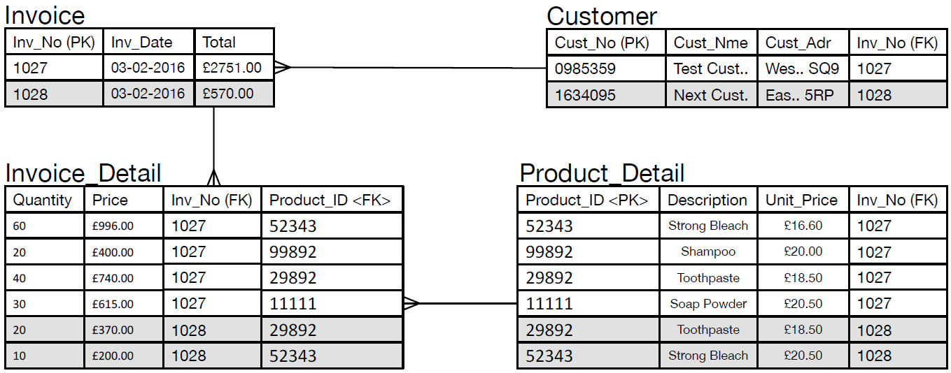
- Figure 12: Final invoice database design.
- The final form of the database, with all included keys and relationships are provided in Figure 12.
-
5.6 Summary
- We covered relational data optimization, a.k.a. ‘normalising relational data’.
- Several ‘anomalies’ we discussed: the ‘update’, ‘insertion’, ‘deletion’ anomalies, before the sequential steps in the process of data optimization were considered. These consist of the process of moving away from an un-normalized to one that is well designed and optimal.
- UNF – 1NF – 2NF – 3NF were covered.
- A scenario concerning a fictional company (G&P Ltd) was presented in order to demonstrate the process of normalization.
- Download PDF Version