07
-
DB Development Essentials: The AMP Stack and MySQL querying
- In this week, we will cover the following topics:
- The architecture of web-based applications.
- Importance of a stack of software to enable web-application development with database interaction (AMP Stack).
- Typical AMP-stack installation flow.
- Further MySQL queries.
- … and will result in the following learning outcomes
- An understanding of the location of various tiers and components in a web-based application.
- Appreciation of what the AMP stack is and why is it important.
- Appreciation of the installation flow for Apache, MySQL, and PHP.
-
7.1 Overview
- This course is called Database Development. In the first part of the course, we have focussed on the principles of relational databases, and we have covered the essential aspects of database design. In the second part of the course, which we begin this week, we start to focus on the practice of relational databases.
- An important part of the practice of relational databases is to get to know your tools:
- SQL QUERIES: We have already seen some very basic SQL commands, in Week 6. SQL commands or ‘queries’ are based, in part, on the underlying principles of databases; more specifically, as we have discussed previously, on some of the mathematical definitions relating to sets. SQL implementations, however, also contain many other features.
- Database Development Environment(s): Database development is usually very much tied up with web application development. It is important, therefore, that you have an understanding of the various software systems available that allow a web application to work, the programming languages related to dynamic web content, and how a database might fit into this picture.
- This week, we will cover some of the key, set-based SQL commands, as well as look at some other features of MySQL. However, given that the development environment is assumed to be in place, for a database developer to use, we will explain a typical kind of software set-up before looking at query language using MySQL. This will provide you, generally, with the context for the second part of the course, which is the practice of relational database systems. Let us briefly remind ourselves of what we will cover in part II, i.e., this week and in weeks 8 and 9:
- The Practice of Relational Database Systems.
- Week 7 (this week): Web DB development environment and Queries.
- Week 8: Server side database programming (with PHP).
- Week 9: Client side database programming (with Java).
-
7.2 Web Applications and the 4 tiers
- Web-based application development consists of numerous components and produces what is therefore known as a multi-tiered application. A multi-tiered application is best thought of as consisting of four separate tiers as follows:
- Client Tier
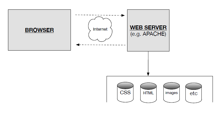
- This consists of the web browser. The web browser is typically installed on a local machine (this can be a desktop computer, a mobile device, a laptop etc. – anything on which you can install a browser). The browser is programmed with an ability to request information from a web server, with two-way communication implying use of HTTP, the foundational protocol for the worldwide-web (WWW) where data is transferred within its physical substrate, the Internet. Browsers have the ability to execute .html mark-up and render the contents visually in the browser for human ‘consumption’.
- Web Tier
- This consists of the HTTP Server. The HTTP server is typically a separate machine which will contain documents and data relating to the static content of a website. Static content refers to content such as .html files, images (that are called/tagged from with the html content) and cascading style sheets (.CSS), files that describe the appearance of the Website in questions. This content is often referred to as static. The Web Server may receive a message from the browser to run an executable script, which is then relayed to the business tier …
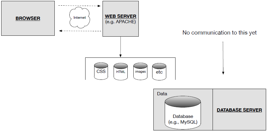
- Business Tier
- This includes an application server. It will receive a message to execute a script/program from the Web Server, upon which it does so and returns a result from the process. During the execution of the script, the program might require access to data. If so, then this part of the process is communicated to a Data Server, in the form of a query.
- Data Tier
- This includes the database server and the database itself. As a consequence of being queried, the Database server will return a response, via communication with the database store, back to the business tier.
- The positioning of all of these components is therefore more complicated than the mere user-interface of the browser. The process as a whole is summarised in Figure 1.
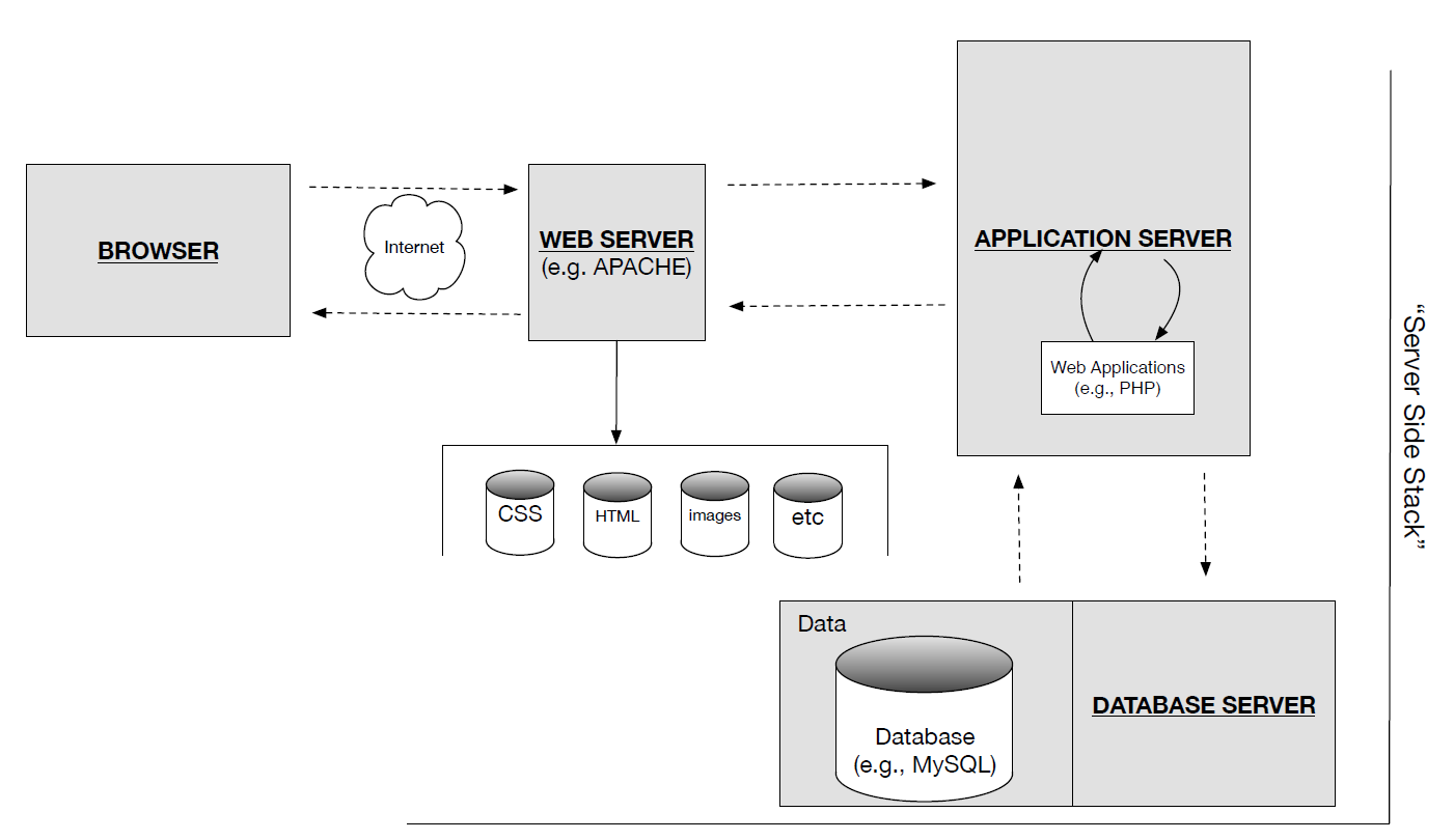
- Figure 1: The browser and the server-side stack.
- The web tier, the business tier and the data tier are known as the server-side stack or server stack. In Table 1 we summarise the technologies typically associated with these tiers, depending on the operating system being used for development – i.e., windows or the Unix based OS’ Mac OS and Linux.
Tier / Server Relevant technologies Web Apache (Windows, Unix)
Internet Information Services (Windows)Business / Application PHP (Windows, Unix)
ASP.net (Windows)Data MySQL (Windows, Unix)
Oracle (Windows, Unix)
SQL Server (Windows)- Table 1: The server stack
- In enterprise development (industrial software settings), different companies will use different development technologies. Nevertheless, the general configuration outlines above will be relevant to many of them running relational databases.
-
7.3 ‘The’ AMP Stack
- The ‘AMP’ prefix to the phrase AMP stack refers to Apache MySQL and PHP. In this section we highlight some of the different installation options that are available. Each one will give you a slightly different AMP stack, but all will allow you to undertake web application development on a local machine.
- Why are we looking into this? As a software developer, database developer, web application developer etc. you will, in an industrial setting be expected to know about the technologies that you are using. Although in some companies a standard, company-wide installation for a given software environment might be available, this is not always the case. Indeed, during your fist days as a software develop or web application developer, you might be asked to “setup you development environment” for the specific role you have been recruited for. You need to get to know the tools you are using.
- In terms of AMP stack installation, there is an excellent resource available on Linda.com. The course Installing Apache, MySQL, and PHP describes in detail…
- “how to install and configure Apache HTTP Server, MySQL database server, and PHP, known collectively as the AMP stack, on a local computer…: installing the components separately on Windows .. Mac…Linux; installing the prepackaged WampServer and MAMP environments; and .. cross platform stacks XAMP and Bitnami”.
Linda.com
- We recommend taking a look at this course and getting interested in the details of the installation and having a think about what each step does. Essentially, the course allows you to set-up your machine to represent the network depicted in Figure 1. That is, it educates in for machine set-up for web application development.
-
7.3.1 AMP stack installation flow (individual components)
- Here, we focus on the installation of individual components which gives you the most insight into configuring your AMP stack, because it is not just a click and install option where everything is done for you. For those interested in following and practicing AMP stack installation we refer you to the aforementioned course.
- It is also useful, on the other hand to see the overall installation flow, and how each different part related to the set-up shown in Figure 1. We therefore provide the installation flow for the AMP stack on Windows, as an example.
-
7.3.2 Example installation flow (AMP individual components on windows)
- A - Install Apache (Web Server)
- 1. Install V C++ Redistributable
- 2. Download Apache and extract to an apache home folder of your choice. For example:
<C:\apache>
- 3. Depending on the location of Apache and the folder name chosen in step 2., configure the httpd.conf file to connect to localhost.
- 4. Start the server. Once done, the server is now in a state in which it can communicate with a web browser
- 5. Browser interface test: type localhost into a browser. If a request is successfully sent to and received from, the server, then “It works!” is rendered by you browser.
- 6. Know your htdocs document root folder. This is the default place for the web content:
- CSSS, HTML, Images, etc.
- The folder is here, assuming the above paths:
<C:\apache\htdocs>
- B - Install (PHP)
- 1. Download PHP to your system
- 2. Extract the contents to a php home folder of your choice. For example:
<C:\php>
- 3. Configure your Apache server to ‘be aware’ of PHP. Relevant changes are made to the following configuration file:
<C:\apache\conf\httpd.conf>
- Test: place a basic php script into the htdocs root folder of Apache server. For example:
<C:\apache\htdocs\phpinfo.php>
- Ensure that the server is running, then call the script from the browser by typing, for example:
<http://localhost/phpinfo.php>
- Into the browser.
- Information should be rendered in the browser.
- At this point you have simulated the browser -web server - communication in Figure 1, as shown.
- Install (MySQL)
- 1. Download and install MySQL community edition, the full size package
- 2. Simply launch the installer and follow the instructions from Lynda.com
- i. Keep the default port 3306
- ii. Set-up a MySQL root account and password
- 3. Launch MySQL Workbench
- i. Connect to the localhost root account instance.
-
7.3.3 Note on ports
- When you install an AMP stack it is important to recognise that the software “listens” (i.e., listens for communication on certain ports). A port is the hardware interface between a computer and other computers.
- Two separate applications should not listen on the same port at the same time. Therefore, if you would like to experiment with different AMP stack installations it is worth knowing this…
- When you use different AMP stacks you should uninstall or ‘turn of’ the ‘other’ AMP stacks on your machine. If you do not do this then AMP Stack in hand is unlikely to install properly and work as should be expected.
-
7.4 SQL Querying
- Logically, we can think of SQL statement types as either part of SQLs Data Manipulation (DML) Language or as part of its Data Definition Language (DDL). Whereas DDL:
- “…allows database objects such as schemas, domains, tables, views, and indexes to be created and destroyed”.
(Connolly and Begg 2015)
- DML refers to:
- “..that part of the SQL language that deals with working with and manipulating data in your table”
(Allardice 2015)
- In practical terms the distinction is not overly important, although it is worth noting that DDL allows you to alter the structure of the actual database etc. While you are developing your SQL skills you will be working interchangeably with data manipulation and data definition. With this in mind the following sections are designed to demonstrate how to
- create a database, named retail_db
- create tables within the database, named Employee and Department
- Select data for viewing
- Sorting data
- Calling SQL aggregate functions
- Joining data
-
7.4.1 Comma-separated test data
- For the following examples we have created two sets of data, stored as .csv files. The structure of the files is fairly well organised, and reflect what you might want to see from a well organised set of data, contained in files stored on a disk. These files relate to Employee data and Department data:
- Header Files:
- <Department_header.csv>.
- Contains the ‘header’ information, the fields names, for the set of columns contained in Department_data.csv. We will draw on the names of these fields when we write a script to create the Department table.
- <Employee_header.csv>
- Contains the ‘header’ information, the fields names, for the set of columns contained in Employee_data.csv. We will draw on the names of these fields when we write a script to create the Employee table.
- Data files:
- <Department_data.csv>
- Contains the actual data of interest with respect to the Department table. We will read this data into our Department table, after it has been created, again using a script.
- <Employee_data.csv>
- Contains the data of interest with respect to the Employee table. We will read this data into our Employee table, after it has been created, likewise using a script.
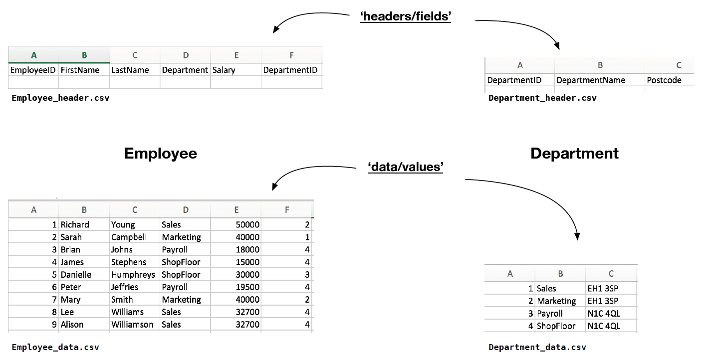
- Figure 2: .csv files 'schemas' and data.
- Our aim is to convert this example .csv data into a MySQL database representation, then run some typical queries over the data and view the outputs. Finally, we will delete the database. These steps will introduce you to some of the typical commands that you will expect to use, and cover aspects of both the DDL and DML aspects of MySQL.
-
7.4.2 Simple Database creation script
Console input
mysql> source create_retail_db.sql;

Console output                            SCRIPT create_retail_db.sql

+-----------------------+                 show database;
|   Database            |                 CREATE DATABASE retail_db;
+-----------------------+                 show databases;
|   Information_schema  |
|   codepoint_db        |
|   mysql               |
|   performance_schema  |
|   sys                 |
+-----------------------+
5 rows in set (0.00 sec)
Query OK, 1 row affected (0.00 sec)

+-----------------------+
|   Database            |
+-----------------------+
|   Information_schema  |
|   codepoint_db        |
|   mysql               |
|   performance_schema  |
|   retail_db           |
|   sys                 |
+-----------------------+
6 rows in set (0.00 sec)
-
7.4.3 Using the created database
- The following sections now assume that we call the following SQL command, which tells SQL that these commands wil apply to the <retail_db> just created. In other words the following commands are within the scope of <retail_db>:
Console input
mysql> use retail_db;

Console output

Database changed
-
7.4.4 Creating the tables
Console input
mysql> source create_department_table.sql

Console output                              Script create department table.sql

Query OK, 0 rows affected (0.02 sec)        CREATE TABLE retail_db.Department(
                                              DepartmentID int(11)
+-----------------------+                     DeptName text,
|   Tables_in_retail_db |                     Postcode text,
+-----------------------+                   ) ENGINE=InnoDB DEFAULT CHARSET=utf8;
|   Department          |                   show tables;
+-----------------------+
1 row in set (0.00 sec)
Console input
mysql> source create_employee_table.sql

Console output                             SCRIPT create employee table.sql

Query OK, 0 rows affected (0.02 sec)       CREATE TABLE retail_db.Employee (
                                             EmployeeID int(11)
+-----------------------+                    FirstName text,
|   Tables_in_retail_db |                    LastName text,
+-----------------------+                    Department text,
|   Department          |                    Salary int(11),
|   Employee            |                    DepartmentID int(11)
+-----------------------+                  ) ENGINE=InnoDB DEFAULT CHARSET=utf8;
2 rows in set (0.00 sec)                   show tables;
-
7.4.5 Loading the tables with data
Console input
mysql> source load_department_data.sql

Console output                             SCRIPT load department data.sql

Query OK, 4 rows affected (0.02 sec)       LOAD DATA LOCAL INFILE '../week-7-data/Department_data.csv'
Records: 4 Deleted: 0 Skipped: 0              INTO TABLE retail_db.Department
Warnings: 0                                     FIELDS TERMINATED BY ','
                                                LINES TERMINATED BY '\n'
Console input
mysql> source load_employee_data.sql

Console output                             SCRIPT load_employee_data.sql

Query OK, 9 rows affected (0.01 sec)       LOAD DATA LOCAL INFILE '../week-7-data/Employee_data.csv'
Records: 9 Deleted: 0 Skipped: 0              INTO TABLE retail_db.Employee
Warnings: 0                                     FIELDS TERMINATED BY ','
                                                LINES TERMINATED BY '\n'
- At this point we are in a position to undertake data manipulation, using MySQL DML commands. Some example commands follow.
-
7.4.6 SQL: Selecting
- In the following example, the SELECT and FROM commands are used. The SELECT word does exactly what it says, and is used to select data from a table. Here, we simply select every (*) column FROM the Employee table.
mysql> SELECT * FROM Employee;

+--------------------------------------------------------------------------------+
|  EmployeeID |  FirstName |  LastName   |  Department |  Salary |  DepartmentID |
+--------------------------------------------------------------------------------+
|           1 |  Richard   |  Young      |  Sales      |   50000 |             2 |
|           2 |  Sarah     |  Campbell   |  Marketing  |   40000 |             1 |
|           3 |  Brian     |  Johns      |  Payroll    |   18000 |             4 |
|           4 |  James     |  Stephens   |  ShopFloor  |   15000 |             4 |
|           5 |  Danielle  |  Humphreys  |  ShopFloor  |   30000 |             3 |
|           6 |  Peter     |  Jeffries   |  Payroll    |   19500 |             4 |
|           7 |  Mary      |  Smith      |  Marketing  |   40000 |             2 |
|           8 |  Lee       |  Williams   |  Sales      |   32700 |             4 |
|           9 |  Alison    |  Williamson |  Sales      |   32700 |             4 |
+--------------------------------------------------------------------------------+
9 rows in set (0.00 sec)
- …and similarly FROM the Department table…
mysql> SELECT * FROM Department;

+-------------------------------------------+
|   DepartmentID |   DeptName  |   Postcode |
+-------------------------------------------+
|              1 |   Sales     |   EH1 3SP  |
|              2 |   Marketing |   EH1 3SP  |
|              3 |   Payroll   |   N1C 4QL  |
|              4 |   ShopFloor |   N1C 4QL  |
+-------------------------------------------+
4 rows in set (0.00 sec)
- SELECT is often also used in conjunction with the WHERE command. WHERE can be used to specify Boolean conditions on the rows that are returned. In the following, for example, the Boolean condition is <Salary > 30000>, such that each row this condition evaluates to ‘true’ is returned from the data. Note the Employees who are missing and their salaries (from the previous displayed Employee table.
- So, as is expected from a query language it is quite easy to return only the specific data you are interested in. We are only using relatively simple examples, here, but you are getting a feel for the powerful nature of query based programming statements. One thing you might want to try, just for fun, is to write a program (say in Java), which reads the same information from the .csv files provided. Otherwise, you can simply trust that the task will be much, much more time consuming and cumbersome that simple executing the statement below.
SELECT * FROM Employee WHERE Salary > 30000;

+--------------------------------------------------------------------------------+
|  EmployeeID |  FirstName |  LastName   |  Department |  Salary |  DepartmentID |
+--------------------------------------------------------------------------------+
|           1 |  Richard   |  Young      |  Sales      |   50000 |             2 |
|           2 |  Sarah     |  Campbell   |  Marketing  |   40000 |             1 |
|           7 |  Mary      |  Smith      |  Marketing  |   40000 |             2 |
|           8 |  Lee       |  Williams   |  Sales      |   32700 |             4 |
|           9 |  Alison    |  Williamson |  Sales      |   32700 |             4 |
+--------------------------------------------------------------------------------+
-
7.4.7 SQL: Sorting
- In the examples that follow, the input commands build on the previous ones by including the use of the ORDER BY words. The first example orders the results by Salary, such that the Salary field determines the order in which the rows appear, in ascending order, from lowest to highest (using the ASC word). The second example used the DESC word, to ensure that the order by salary is in descending order. Notice, if you omit ASC (or DESC) then the default is ascending.
SELECT * FROM Employee WHERE Salary > 30000 ORDER BY Salary;
SELECT * FROM Employee WHERE Salary > 30000 ORDER BY Salary ASC;

+--------------------------------------------------------------------------------+
|  EmployeeID |  FirstName |  LastName   |  Department |  Salary |  DepartmentID |
+--------------------------------------------------------------------------------+
|           8 |  Lee       |  Williams   |  Sales      |   32700 |             4 |
|           9 |  Alison    |  Williamson |  Sales      |   32700 |             4 |
|           2 |  Sarah     |  Campbell   |  Marketing  |   40000 |             1 |
|           7 |  Mary      |  Smith      |  Marketing  |   40000 |             2 |
|           1 |  Richard   |  Young      |  Sales      |   50000 |             2 |
+--------------------------------------------------------------------------------+
5 rows in set (0.01 sec)
SELECT * FROM Employee WHERE Salary > 30000 ORDER BY Salary DESC;

+--------------------------------------------------------------------------------+
|  EmployeeID |  FirstName |  LastName   |  Department |  Salary |  DepartmentID |
+--------------------------------------------------------------------------------+
|           1 |  Richard   |  Young      |  Sales      |   50000 |             2 |
|           2 |  Sarah     |  Campbell   |  Marketing  |   40000 |             1 |
|           7 |  Mary      |  Smith      |  Marketing  |   40000 |             2 |
|           8 |  Lee       |  Williams   |  Sales      |   32700 |             4 |
|           9 |  Alison    |  Williamson |  Sales      |   32700 |             4 |
+--------------------------------------------------------------------------------+
5 rows in set (0.00 sec)
- When you order a text value, such as Department field, then the default is ascending alphabetic order:
SELECT * FROM Employee WHERE Salary > 30000 ORDER BY Department;

+--------------------------------------------------------------------------------+
|  EmployeeID |  FirstName |  LastName   |  Department |  Salary |  DepartmentID |
+--------------------------------------------------------------------------------+
|           2 |  Sarah     |  Campbell   |  Marketing  |   40000 |             1 |
|           7 |  Mary      |  Smith      |  Marketing  |   40000 |             2 |
|           1 |  Richard   |  Young      |  Sales      |   50000 |             2 |
|           8 |  Lee       |  Williams   |  Sales      |   32700 |             4 |
|           9 |  Alison    |  Williamson |  Sales      |   32700 |             4 |
+--------------------------------------------------------------------------------+
5 rows in set (0.00 sec)
- It is also possible to order by one column (primary ordering column), and then by another (secondary ordering column). For instance, in the following example, we order primarily by Department, so we get the same ordering in the Department column, but because we then order by LastName, the order of the rows can be seen to alter according to this field within. The set of ‘Sales’ Employees:
SELECT * FROM Employee WHERE Salary > 30000 ORDER BY Department, LastName;

+--------------------------------------------------------------------------------+
|  EmployeeID |  FirstName |  LastName   |  Department |  Salary |  DepartmentID |
+--------------------------------------------------------------------------------+
|           2 |  Sarah     |  Campbell   |  Marketing  |   40000 |             1 |
|           7 |  Mary      |  Smith      |  Marketing  |   40000 |             2 |
|           8 |  Lee       |  Williams   |  Sales      |   32700 |             4 |
|           9 |  Alison    |  Williamson |  Sales      |   32700 |             4 |
|           1 |  Richard   |  Young      |  Sales      |   50000 |             2 |
+--------------------------------------------------------------------------------+
5 rows in set (0.00 sec)
- Any number of separate ordering can be done in this nested way, which makes it very useful for organising large amounts of rows.
-
7.4.8 SQL: Functions
- Where we are not necessarily interested in the specific details of the data itself, we might want to use some of the aggregate functions available in MySQL. These functions allow us to count, find minimum, maximum and average values on those aspects of the data we are interested.
- For a very simple example, you can simply count the number of rows in a table…
SELECT COUNT(*) FROM Employee;

+------------+
|   COUNT(*) |
+------------+
|         9  |
+------------+
1 row in set (0.01 sec)
SELECT COUNT(*) FROM Department;

+------------+
|   COUNT(*) |
+------------+
|         4  |
+------------+
1 row in set (0.00 sec)
- Or, if you are interested in counting a subset of the data (like the number of Employees who earn over 30000) you can count on this subset.
SELECT COUNT(*) FROM Employee WHERE Salary > 30000;

+------------+
|   COUNT(*) |
+------------+
|         5  |
+------------+
1 row in set (0.00 sec)
- Min and Max can be used. Who earns the least…
SELECT MIN(Salary) FROM Employee;

+---------------+
|   MIN(Salary) |
+---------------+
|         15000 |
+---------------+
1 row in set (0.00 sec)
- …and who earns the most…
SELECT MAX(Salary) FROM Employee;

+---------------+
|   MAX(Salary) |
+---------------+
|         50000 |
+---------------+
1 row in set (0.00 sec)
- What the total salary of all employees is:
SELECT SUM(Salary) FROM Employee;

+---------------+
|   SUM(Salary) |
+---------------+
|        277900 |
+---------------+
1 row in set (0.01 sec)
- the average…
SELECT AVG(Salary) FROM Employee;

+---------------+
|   AVG(Salary) |
+---------------+
|   30877.7778  |
+---------------+
1 row in set (0.00 sec)
The following use of the function count is undertaken on a set of groups, grouped by salary.
SELECT COUNT(Salary), Salary FROM Employee GROUP BY Salary;

+----------------------------+
|  Count(Salary) |   Salary  |
+----------------------------+
|              1 |     15000 |
|              1 |     18000 |
|              1 |     19500 |
|              1 |     30000 |
|              2 |     32700 |
|              2 |     40000 |
|              1 |     50000 |
+----------------------------+
7 row in set (0.00 sec)
-
7.4.9 SQL: Joining
- When we created the database, above, we created two tables. However, as we have seen in earlier parts of the course, the idea behind database organisation, isn’t just to separate logically related data, but to then allow separate tables to be related to each other.
- A key SQL table command for this is the JOIN command. This allows us to join two tables together. In the following example, we select FirstName, LastName and DeptName. Note, FirstName and LastName are fields within the Employee table. DeptName is a field within the Department table. However the geneal <SELECT contents FROM table> syntax works on a table which is the joined table of Employee and Department. You can think of this as a table that exists as a consequence of the JOIN. In this case, the join is made on (ON) the DepartmentID of both the Employee and the Department tables.
SELECT FirstName,LastName,DeptName FROM Employee INNER JOIN Department ON Employee.DepartmentID = Department.DepartmentID;

+--------------------------------------------+
|   FirstName  |   LastName  |   DeptName    |
+--------------------------------------------+
|   Richard    |   Young      |   Marketing  |
|   Sarah      |   Campbell   |   Sales      |
|   Brian      |   Johns      |   ShopFloor  |
|   James      |   Stephens   |   ShopFloor  |
|   Danielle   |   Humphreys  |   Payroll    |
|   Peter      |   Jeffries   |   ShopFloor  |
|   Mary       |   Smith      |   Marketing  |
|   Lee        |   Williams   |   ShopFloor  |
|   Alison     |   Williamson |   ShopFloor  |
+--------------------------------------------+
9 rows in set (0.00 sec)
-
7.5 Summary
- We covered a topic related to web applications, and the various software tiers relevant - ‘client’, ‘web’, ‘business’, ‘data’.
- Following on from last week, covered something known as the AMP stack, and briefly the main steps of the AMP stack installation flow.
- Following this introduced SQL querying with the number of Basic MySQL commands to create a database, create tables with a database, select, sort data, and join data tables together.
- Download PDF Version