Wk 2
Shear Force and Bending Moment Diagrams
- A beam is a structure that is subjected to external forces where, in most cases, beams are horizontal and the loads they carry act vertically downwards, perpendicular to the longitudinal axis.
This lecture will show how to draw thrust, shear force and bending moment diagrams for beams carrying more complex loading including a combination of vertical point loads, inclined point loads, uniformly distributed loads, non-uniformly distributed loads and couple effects.- A beam is a structure that is subjected to external forces where, in most cases, beams are horizontal and the loads they carry act vertically downwards, perpendicular to the longitudinal axis.
- Figure 1 (cont.)
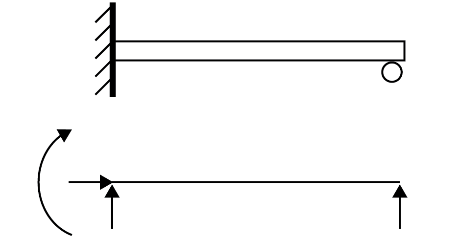 Built-in at one end, simply-supported at the other (propped cantilever)
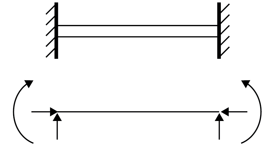 Built-in at both ends (encastre beam)
- Equilibrium of Beams
The algebraic sum of all the forces acting on the beam (including reactions) is zero [in the horizontal (x) and vertical (y) directions)], and the sum of all moments acting about any point is zero, i.e.
For a beam to be at rest (i.e. in equilibrium) when acted upon by external forces, the conditions of 2 dimensional equilibrium must be satisfied:
$$ \large \sum F_x = 0 $$ $$ \large \sum F_y = 0 $$ $$ \large \sum M_A = 0 $$
Shear Force & Bending Moments
- In order to carry external forces, a beam has to be placed on supports which provide reactions to the external actions. The types of supports commonly used are:
1. knife edges, rollers or pins (simply-supported beam).
2. built-in at one end (cantilever beam).
3. built-in at one end, simply-supported at the other (propped cantilever).
4. built-in at both ends (encastre beam).
Figure 1 below shows examples of the beams described in 1 – 4 above and their associated free-body diagrams
Figure 1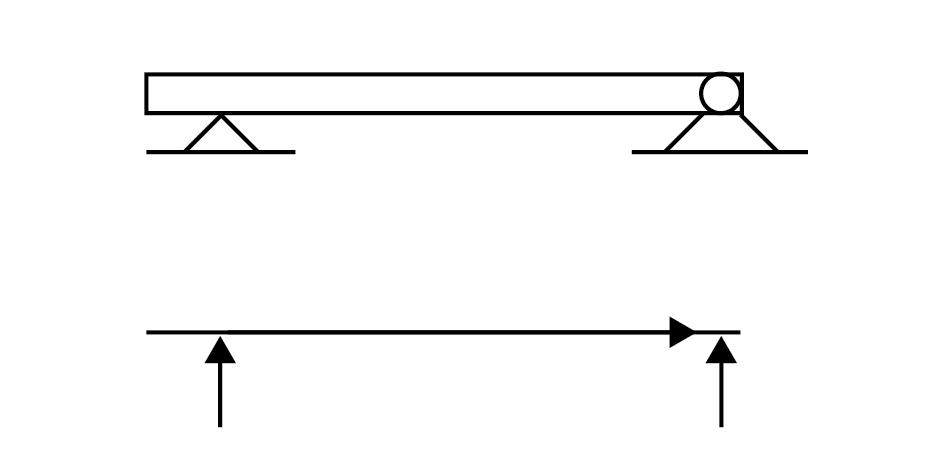 Knife edges, rollers or pins (simply-supported beam)
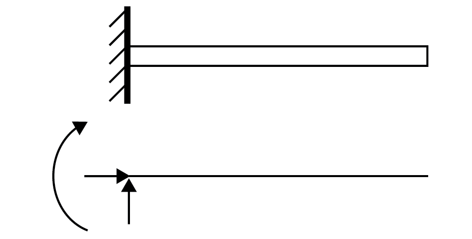 Built-in at one end (cantilever beam)
- Equilibrium of Beams
- General Rules
1. In the absence of distributed loads (UDLs), the SF diagram consists of horizontal steps and the BM diagram is a series of straight lines.
2. For a beam (or part of a beam) carrying a UDL only, the SF diagram is a sloping straight line and the BM diagram is a parabola.
3. At a point where the SF diagram passes through zero (i.e. where the SF changes sign), the BM diagram has a maximum or minimum value.
4. Over a part of the span for which SF is zero, the BM has constant value.
5. At a point where the BM = 0, this is called a point of contraflexure (or inflexion).
- Application of 2 Dimensional Equilibrium to Beams
Consider the beam shown in Figure 3 which shows a simply-supported beam with 4 external point loads acting upon it.
Figure 3
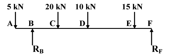
For equilibrium of forces, the sum of the four external vertical forces acting downwards must be equal to the sum of the two reaction forces acting vertically upwards, i.e.
$ \sum F_y = 0 \therefore $ -5 + R $ _B $ – 20 – 10 – 15 + R $ _F $ = 0 or R $ _B $ + RF = 50 kN (i)
Equation (i) above cannot be solved since there are two unknown forces R $ _B $ and R $ _F $.
Continues on next tab (1.3)
Shear Force & Bending Moments
- Types of Load
There are two main types of loading which act on beams: concentrated or point loads that are applied to the beam through a ‘knife-edge’ and are shown on diagrams by arrows – point loads can be inclined at any angle to the beam causing a horizontal thrust; uniformly distributed loads (UDL) are spread over the whole or part of a beam so that the load carried by a given portion is proportional to the length of that portion – these can be uniform and/or non-uniform. The magnitude of a UDL is measured in N/m and is usually denoted by $ \omega $.
Figure 2 shows examples of beams with point loads and UDLs. Moments can also be applied at any point on a beam and can be clockwise or anticlockwise in direction.
Figure 2 Point Loads
 Point Loads/UDL
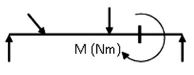 Point Loads/Moment
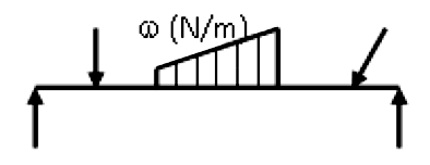 Point Loads/Varying UDL
- General Rules
- *Notes:
1. Where the SF values change from +ve to –ve (at points B and D in this case) indicates the position where the maximum bending moment occurs (-5 kNm maximum anticlockwise moment at B; 45 kNm maximum clockwise moment at D).
2. Where the bending moment values change from +ve to –ve (between points B and C in this case) indicates a point of contraflexure where M=0. The exact position of this point can be found by deriving a moment equation about the point, i.e. for this example, let’s say the point of contraflexure occurs at x (m) to RHS of point A:
$ \sum M_x $ = 0 = -5x + 27.5(x-1) $ \;\; \therefore\; \;$ x = 1.22 m
- From the diagram in figure 5, the maximum shear force is 22.5 kN along portions BC and EF, and the maximum bending moment is 45 kNm acting at D.
To calculate the bending moments, use can be made of the shear force diagram:
area AB = moment at B;
area AB+BC = moment at C;
area AB+BC+CD = moment at D (maximum in this case);
area AB+BC+CD+DE = moment at E;
area AB+BC+CD+DE+EF = moment at F (= 0 in this case)
Alternatively, moment equations can be derived to calculate the magnitude of the bending moment at each point, i.e.
-(5x1) = -5 kNm;
-(5x3)+(27.5x2) = 40 kNm;
-(5x5)+(27.5x4)-(20x2) = 45 kNm;
-(5x8)+(27.5x7)-(20x5)-(10x3) = 22.5 kNm;
-(5x9)+(27.5x8)-(20x6)-(10x4)-(15x1) = 0 kNm.
Continued from previous tab (1.2)Consider the same beam with the distances between each of the points as shown in Figure 4.
Figure 4For equilibrium of moments, the sum of the moments caused by all forces must be equal to zero at any point along the beam. However, to have an equation containing just one unknown reaction force, moments are taken about B (noting that +M is clockwise and –M is anticlockwise), i.e.
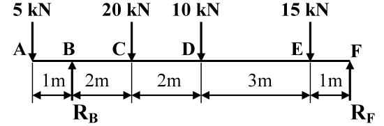
$ \sum M_B = 0: \; \therefore $ -(5x1) + (20x2) + (10x4) + (15x7) – (8xR$_F$) = 0 $ \therefore $ R F = 22.5 kN
Hence substitute R$_F$ = 22.5 kN in Eqn.(i) above gives:
RB + 22.5 = 50 $ \therefore $ R B = 27.5 kN
- Shear force (SF) and bending moment (M) diagrams can be drawn that show their variation along the span of the beam:
Figure 5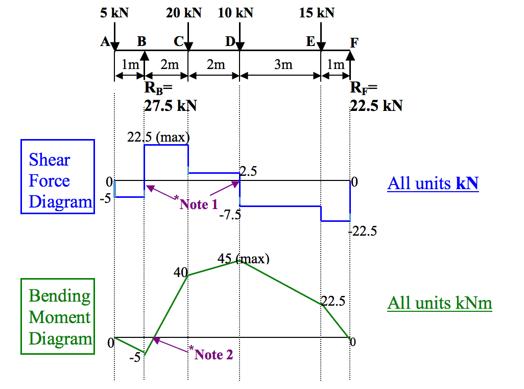
- *Notes:
- Point Loads and UDLs
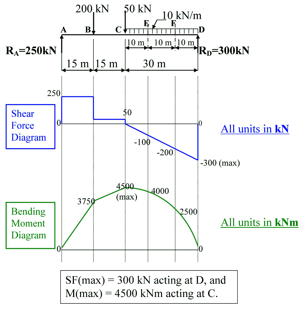
The beam analysed above was acted upon by point loads only. Figure 6 shows a beam with both point loads and a UDL acting upon it.
Figure 6
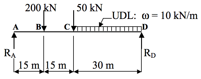
Reactions at A and D:
$ \sum M_A = 0$: (200x15) + (50x30) + [(10x30)x45]-(60xR$_D$) = 0 $ \; \therefore \; $ RD = 300 kN
$ \sum F_y = 0$: RA –200 - 50 - (10x30) + 300 = 0$ \; \therefore \; $ RA = 250 kN- Point Loads and UDLs
-
Summary
- ⬇ Summary
-
Tutorials
- ⬇ Tutorial