-
 Chapter 3 - 5, Math Bollen And Fainan Hassan - Integration of Distributed Generation in thePower System
Chapter 7, Jenkins, N., etc. “Distributed Generation” R
Unit Overview
In this unit, you will learn :
- The concept of power flow analysis and its application to a distribution network
- How DG may affect losses in a distribution network.
- How to estimate the hosting capacity of DG against feeder overloading in a distribution network.
- How to increase the hosting capacity against feeder overloading.
-
Introduction to Power Flow Analysis for a Distribution Network
Power-Flow Analysis
- Power flow analysis is probably one the most frequent job for the daily plan of a power system.
- It is also referred to as “load flow analysis”
- Power flow analysis is commonly used to estimate the steady-state condition of an AC power system
- Variables for calculation in power flow analysis include: bus voltage magnitudes (voltage), bus phase angles (angles), the flow of active power (P) and reactive power (Q) out of a node or through a circuit branch
- Power flow cannot be used to assess the dynamics or transients of a power system because it assumes the power system is under steady-state conditions: the system is operating at nominal frequency (e.g. 50 Hz in UK)
The Applications of Power-Flow Analysis
Why power flow analysis?
- Power system planning and design
- Power system steady-state operation monitoring: losses, voltage profiles, feeder loading, etc.
- Analysis for
– Stability: power flow analysis is the first step to determine the operational point before carrying out small signal analysis for dynamics
– Fault analysis: power flow analysis can tell the fundamental components of fault currents, in other words, the steady state fault current.
Power-Flow Approach
- For power flow analysis, the entire electrical network is defined as nodes in connection with power lines and transformers. All the elements involved follows certain modelling patterns:
– Most generators: normally modelled as a source of active power and voltage called “PV node”
– The “slack” generator: as a voltage source to balance the power flow, source of voltage and reference angle (often 0 for simplicity), “slack node” or “balance node”
– Load: normally a source of active power and reactive power, “PQ node”; some generator with reactive regulation can also be modeled as PQ node, e.g. PV arrays.
– Power lines and transformers: Impedance (or admittance)
– Once all the electrical elements are modelled in an electrical network, equations can be set up and solved using the generic approaches of circuit analysis. Nowadays, it is carried out by computers in daily practice.- Could the power flow equations be solved by linear circuit analysis approach? – No.
– Power flow equation is completely non-linear, which cannot be solved with a generic analytical solutions.
– It can only be solved using numerical approach.
– Special iteration technique need to be used and it is usually performed by a computer.
– There are a variety of power flow analysis software in the market.
Example of Power Flow modelling
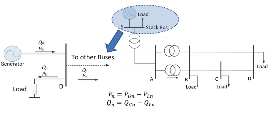
A 5- node system is illustrated. Node 1 is defined as a slack node (bus), which consists of a generator and a load. The power of the node is net power of the generation and load as described by the equations above.
- The slack bus in a power system is assumed with unchanged voltage magnitude and its angle is set at 0.
- Usually the slack bus is selected as the generator bus with the largest power capacity or the substation bus that is unlikely affected by the change in the downstream network.
Steps for Power Flow Analysis:
The load flow analysis with the aid of a computer software can be generically divided into the following steps
- Gathering data : (generators , transformers, lines, cables, loads, etc.) in per unit
- Creating a model (system elements and topology)
- Setting up cases: (load and generation conditions, position of transformers taps and setting of other control devices)
- Solve the system (Running the program)
- Analyzing the results
There are now a variety of power flow analysis software package in market. The implantation may vary, but the general procedures are largely the same.
Power System with DG: Creating an Example Model with a benchmark system
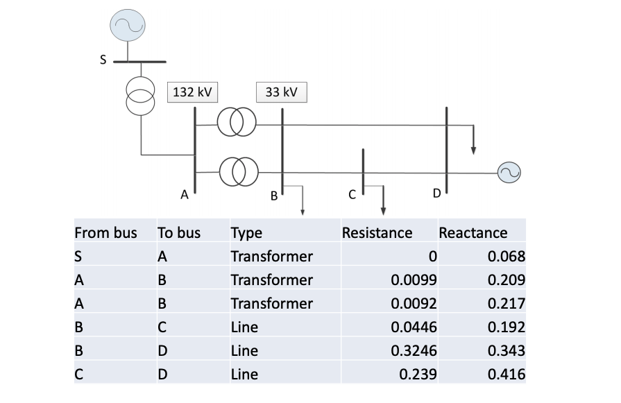
Once the network is established, the power line impedances can be input as illustrated below, where it depicts a complete power system from the power station to 132 kV transmission system, substation to 33 kV and the downstream distribution network. To make the case simple, per unit values are used for the network impedance values.
Case 1: Power Flow Distribution without DG
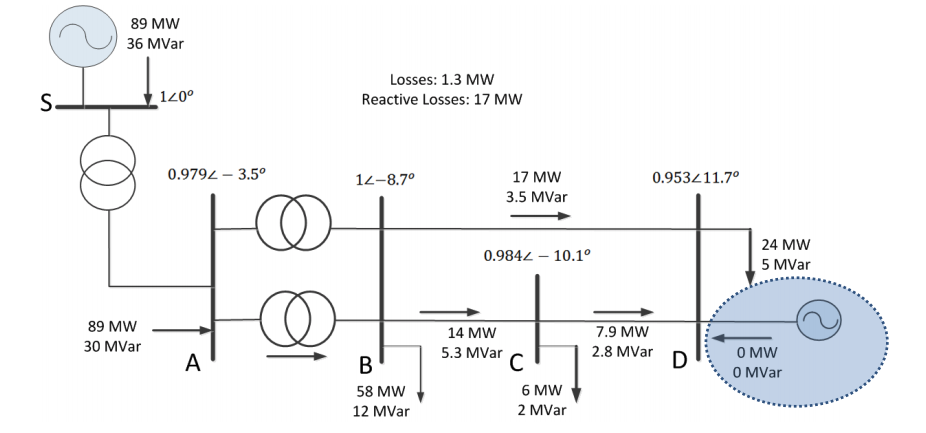
- The power flow distribution for case 1 as an initial case study is shown above, where no DG power is generated.
- It can be seen that all the load flows in the power lines are towards the downstream bus D.
- The bus voltages are expressed in per unit; whereas the power flows are in real value.
- It can also be seen that since the power flow is uni-directional, the voltage at the downstream buses are generally lower than the upstream (the power plant on the top left side)
Case 2: Power System with Significant DG Active Power (0 reactive power)
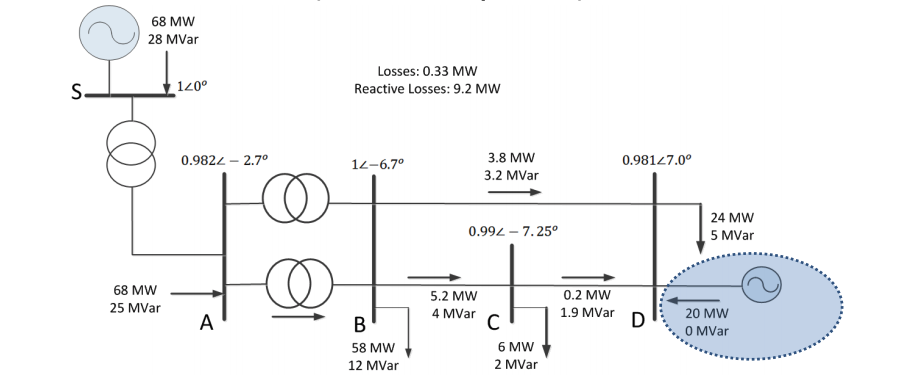
- The power flow distribution for case 2 is shown above, where a significant DG is connected with 20 MW generation.
- It can be seen that although the directions of power flows are not changed comparing to Case 1 (due to the heavy load), but values of power have been significantly reduced.
- This reduction not only reduce the loading stress on all the power lines, but reduce the power distribution losses by approximately 1 MW as well.
- Case 2 demonstrates that a DG can significantly reduce distribution losses when consumed locally!
Case study – The Impact of Active Power Generation of DG
As the comparison shown by Case 1 and 2:
- The cause of difference is in that the DG generation is 0 MW in Case 1 and 20 MW in Case 2
- With active distributed power generation, the voltage profile is higher. (example: voltage of Bus D from 0.953 to 0.981 p.u. )
- Losses are considerably lower in Case 2 because
– Generation closer to the loads so no transmission losses
– Voltage drops over distribution lines reduced; meanwhile the line impedance unchanged
– The apparent currents carried by all the power lines are reduced; hence less losses consumed by the power lines
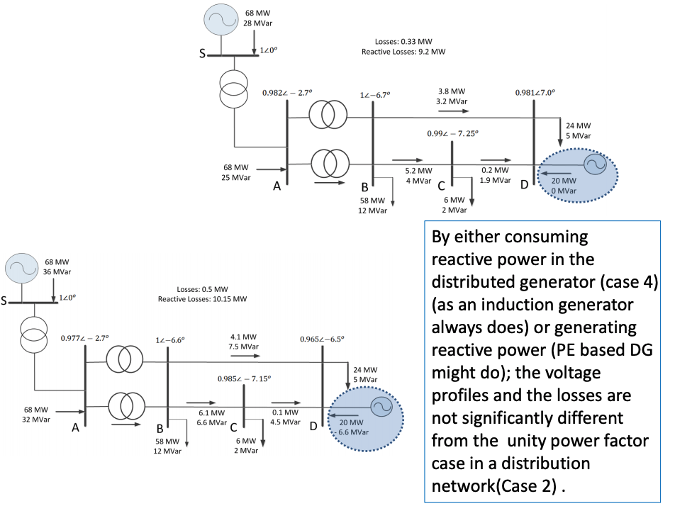
Case 3: Power System with Significant Active Power and Reactive power from DG
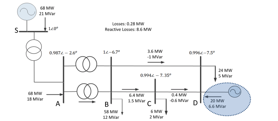
- Based on Case 2, a significant reactive power generation of 6.6 MVar is injected into the power grid by the DG in Case 3.
- It can be seen that although the reactive power generation is quite significant, the voltage profile of the buses has only been leveled up insignificantly.
- Consequently, the losses are further reduced to a very limited extend.
- Since the power lines in a distribution network is more resistive than the transmission, the impact of reactive power against voltage and loss profile is less significant.
Case study – The Impact of Embedded Reactive Power Generation
As the comparison shown between Case 2 and 3:
- The cause of difference is that the reactive power generation of the DG is 0 MW in Case 2 and 6.6 MW in Case 3
- With more reactive distributed power generation, the voltage profiles of all the buses are slightly higher. (example: voltage of Bus D from 0.981 to 0.996 p.u. )
- Losses are slightly reduced by the distributed reactive power generation
- Because the power lines in medium voltage and low voltage is relatively less inductive
– The Voltage drops over distribution lines reduced only slightly but demand a quite significant power capacity from the DG side
– The system optimization using reactive power in distribution network is less effective than in transmission level
Case 4: Power System with Significant Active Power Generation and Reactive Power Absorption from DG
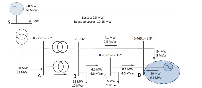
- Based on Case 2, a significant reactive power consumption is absorbed from the distribution network by the DG along with the 20 MW active power generation in Case 4.
- It can be seen that although the reactive power consumption is considerable, the voltages of the buses has only be decreased insignificantly.
- Consequently, the losses are increased slightly.
- Again, thanks to the more resistive nature in a distribution network, the impact of extra reactive power demand will not degrade the voltage profile and efficiency much.
Case 5: Power System with Significant Active Power Generation and Light Load
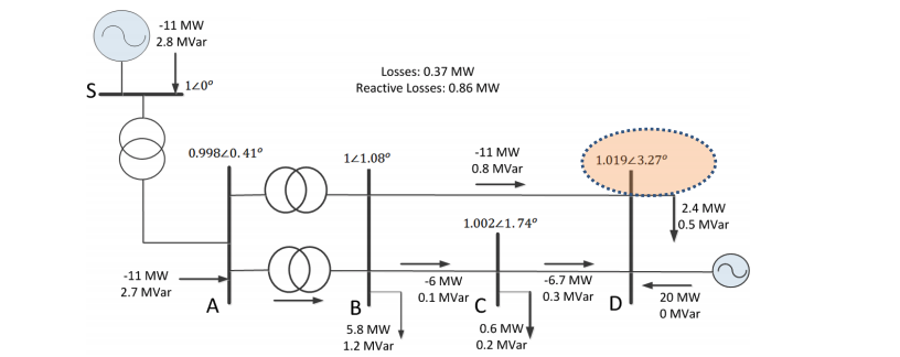
- Based on Case 2, all the loads in the distribution network has been reduced by 90% in Case 5.
- As a result, the 20 MW active power generation exceed the local loads.
- It can be seen that all the power flow carried by the power lines are reversed (noted by negative values).
- Although the distribution losses are still small, but the reverse power flow, at 11MW, must be consumed somewhere of a another distribution network in the power system, whose losses are not counted in this model.
- A significant feature is that such reverse power flow also cause a higher voltage at the end bus of a distribution network (Bus D) than the transmission side (in per unit).
Case Study: full load with DG V.s. Light load with DG
As the comparison shown between Case 2 and 5:
- The cause of difference is the significant reduction of the local loads.
- Since the DG is higher than all the local loads of the distribution network, the active power reverses back to the transmission system.
- Losses are still low in the distribution network, but the possible losses in the transmission system is not counted in this case study. Practically, this can be considerable.
- The reverse power flow also causes a clear voltage rise on the DG side (end side), which means there could be a potential risk of over-voltage if the loads drops further or the DG generation goes higher
-
DG and Losses
DG and Losses - 1
- Impact of DG (small amount of DG)
- DG of smaller scale (roof top PV, small wind turbine, domestic CHPs) is connected closer to the loads than conventional large-scale generation.
- By delivering the same amount of power, a shorter distance simply means i 2R losses are lower.
- Obviously, the best scenario, for the reduction of power line i 2R loss, is to have the DG at exact the same premises of the loads.
- On the other hand, DG also means the load flow from centralized power plant to the loads is reduced.
- In terms of the load flow direction from upstream to downstream, the risk of overloading is increased.
DG and Losses - 2
- For any power system, it can be generally concluded that if the all the power DGs generate is supplying local loads, the losses are minimized and it is always good to have the DG consumed locally.
- For DGs that outweighed the local consumption, distribution losses will again rises. Comparing with transmitting and distribution power all the way from central power plant, such losses are still limited.
- For the case when DG exceeds the local load, assuming that the load and generation have similar profile in time for all feeder sections, as long as the average generation (𝐺𝑚𝑒𝑎𝑛) is less than twice the average load (𝐿𝑚𝑒𝑎𝑛) , no significant increase in losses will be expected, which can be expressed as
𝐺𝑚𝑒𝑎𝑛 < 2𝐿𝑚𝑒𝑎𝑛
Power flow analysis can be employed for more accurate estimation with more complex cases, which may concern system operation.
Further Reading - Chapter 4.4 , Math Bollen And Fainan Hassan - Integration of Distributed Generation in the Power System
DG and Losses - 3
- If the increase in losses is a result of extra DG generation, it is normally not a major concern.
- The percentage of losses is normally limited comparing with the maximum generation capacity allowed.
- From an environmental viewpoint, the gain from renewable energy is much higher than the increase in losses, which produces a significant net income of power.
- For most cases, the issue of overload is more critical than a minor increase of losses as it may end up as a trip, which will degrade the power supply reliability.
- For the extreme case that DGs are large enough to reverse the net power flow of a distribution network to the transmission level, it may become a completely different story, as it is normally not expected by the Transmission System Operators (TSO). The further losses to transmit the power to be consumed by another distribution network can be considerable.
-
Hosting Capacities against the Feeder Overloading
Hosting Capacity (HC)
- The integration of DG itself can sometimes improve the performance of a power system while in other cases deteriorate it, which is illustrated below. “Performance Indicators” measures the performance of power system when a certain element is introduced to the power system.
- There can be a number of indices that are affected by the capacity of DGs that is hosted and the impact of a certain DG may increase the value of certain index at the same time.
- As an illustration, the growing HC is driving one performance index towards the lower limit on the down left figure; the growth might be driving another index towards the upper limit on the down right side at the same time.
- When a performance indicator has reached a forbidden limit due to the capacity of a DG, a Hosting Capacity (HC) is reached. E.g. in the down left, it refers to “HC1”; down right, “HC2”
- There can be many HCs for a certain DG scheme, but the lowest one is the determinative one.
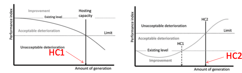
Image: by Chapter 3, Math Bollen And Fainan Hassan - Integration of Distributed Generation in the PowerSystem
Hosting Capacity Approach
The determination of HC may follow a generic approach as follows:
- Pick up a location for DG installment.
- Choose a phenomenon and one or more performance index that is likely to be deteriorate to examine (example: voltage, loading, etc.)
- Determine a suitable limit or limits of the index
- Calculate the performance index as a function of the amount of generation
- Obtain the corresponding HC value when the index has reached a pre-defined limit
- Repeat the previous process with other index and make decision accordingly
Please read Chapter 3.3, Math Bollen And Fainan Hassan - Integration of Distributed Generation in the Power System
Overloading in Radial Distribution Network: the 1st Hosting Capacity
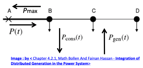
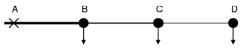
Considering a radial network on the left.
Before DGs are installed, the power flows from A to D at P(t).
The total load fed from A is Pcons(t).
After installing DGs, the total generation power is Pgen(t).Therefore, there is 𝑃 𝑡 = 𝑃𝑐𝑜𝑛𝑠 𝑡 − 𝑃𝑔𝑒𝑛(𝑡)
Since P(t) will not exceed Pcons(t) as long as Pgen(t) is smaller than Pcons(t), the loading of the feeder will not be lighter in such scenario; and the only possibility of overload is when the generation exceed the load.
If the feeder capacity is considered to be designed for the maximum load level, the maximum reverse power Pmax should follow: 𝑃𝑚𝑎𝑥 < 𝑃𝑐𝑜𝑛𝑠,𝑚𝑎x
- The maximum reverse power flow occurs when the maximum generation and minimum consumptions are reached and it can be described as
𝑃𝑚𝑎𝑥 = 𝑃𝑔𝑒𝑛,𝑚𝑎𝑥 − 𝑃𝑐𝑜𝑛𝑠,𝑚𝑖x , which is also referred to as the “First Hosting Capacity” (1st HC).
The corresponding HC is 𝑃𝑔𝑒𝑛,𝑚𝑎𝑥 = 𝑃𝑐𝑜𝑠,𝑚𝑎𝑥 + 𝑃𝑐𝑜𝑠,𝑚𝑖x
The 1st HC for B,C and D can be calculated in a similar way.
Overloading in Radial Distribution Network: the 2nd Hosting Capacity
- If the limit for the reverse power is set to be the thermal limit of the feeder Pmax,limit, there is
𝑃𝑔𝑒𝑛,𝑚𝑎𝑥 − 𝑃𝑐𝑜𝑠,𝑚𝑖𝑛 < 𝑃𝑚𝑎𝑥,𝑙𝑖𝑚𝑖t
The corresponding HC becomes
𝑃𝑔𝑒𝑛,𝑚𝑎𝑥 = 𝑃𝑚𝑎𝑥,𝑙𝑖𝑚𝑖𝑡 + 𝑃𝑐𝑜𝑠,𝑚𝑖x,
which is called the “Second Hosting Capacity” (2nd HC).- The difference between the 1st and 2nd HC is the set limit of the reverse power.
- Considering the designed maximum load is always lower than the feeder thermal limit, the 1st capacity is a rather conservative estimation of HC.
- The 2nd HC is the actually HC that may cause a network trip, since the nominal value of a feeder protection is more likely to be the actual thermal limit, which will degrade the system power distribution reliability.
Example 1: Overloading in a Radial Network
Consider the feeder shown with conductor and consumption data in the table below. The ampacity values are for underground cables. A nominal voltage equal to 15 kV has been used to calculate the maximum permissible (apparent) power from the ampacity.
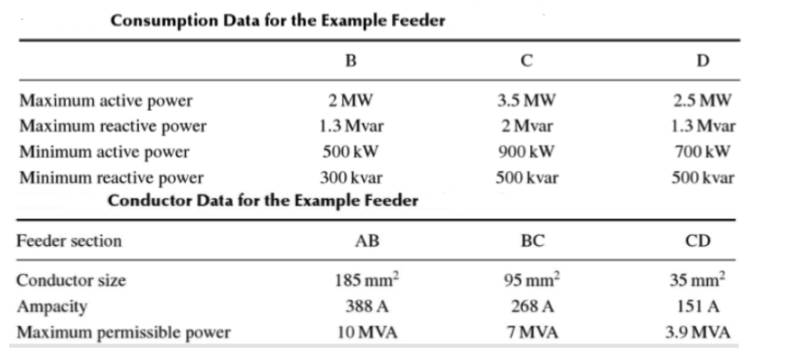
- The first Hosting Capacity (HC) for feeder section CD is 𝑃𝑔𝑒𝑛,𝑚𝑎𝑥 = 𝑃𝑐𝑜𝑠,𝑚𝑎𝑥 + 𝑃𝑐𝑜𝑠,𝑚𝑖𝑛= 2.5 MW + 700 kW = 3.2 MW
- For feeder section BC, all the downstream load should be considered, that is, Load C and Load D. The first hosting capacity is 𝑔𝑒𝑛,𝑚𝑎𝑥 = 𝑃𝑐𝑜𝑠,𝑚𝑎𝑥 + 𝑃𝑐𝑜𝑠,𝑚𝑖𝑛= (2.5+3.5) MW+ (700+900) kW = 7.6 MW
The possible allocation of HC 1 for each load point will be (as a conservative estimation)
D: 3.2 MW
C: 7.6-3.2 = 4.4 MW
B: 10.1 – 7.6 =2.5 MW
- The 2nd Hosting Capacity (HC 2), when the actual overload happens, for feeder section CD is 𝑃𝑔𝑒𝑛,𝑚𝑎𝑥 = 𝑃𝑐𝑜𝑠,𝑙𝑖𝑚𝑖𝑡 + 𝑃𝑐𝑜𝑠,𝑚𝑖𝑛= 3.9 MW + 700 kW = 4.6 MW
- For feeder section BC, the sum of the maximum power of this section and the minimum of all down stream consumption gives the second hosting capacity 𝑃𝑔𝑒𝑛,𝑚𝑎𝑥 = 𝑃𝑐𝑜𝑠,𝑙𝑖𝑚𝑖𝑡 + 𝑃𝑐𝑜𝑠,𝑚𝑖𝑛= 7 MW + (700 +900)kW = 8.6 MW
- For feeder section AB the HC2 is 𝑃𝑔𝑒𝑛,𝑚𝑎𝑥 = 𝑃𝑐𝑜𝑠,𝑙𝑖𝑚𝑖𝑡 + 𝑃𝑐𝑜𝑠,𝑚𝑖𝑛= 10 MW + (700 +900+500)kW = 12.1 MW
-
Increasing Hosting Capacity Against Overloading
Increasing the Hosting Capacity - 1
As is fore cited, the DG generation can significantly improve system efficiency, provided it does not exceed the local loads. Since the DG in most areas are still limited, the main issue for most of the distribution networks is how to increase the hosting capacities against feeder overloading?
- The first thought is always to increase the size of feeders.
● Using wires with a larger cross section area so the thermal rating can be increased.
● Alternatively, adding a new line in parallel can be a practical option.
● This is clearly a costly option for most cases.- Building new connection to provide extra path for the DG can be another option.
● Again costly.
● This may include the upgrade of the protections as it may change the network configuration hence the fault behavior as well.
Increasing the Hosting Capacity - 2
- Use of Intertrip schemes
● The DG will be disconnected once the undesirable network configuration changes, e.g. large load switched out.
● Result in economical losses to the renewable DG owner
● The scheme is very complex and not very practical if there is a large number of small scale DGs- Energy Management System (EMS) with advance protection system
● At every instant, the maximum amount of generation that can be injected is calculated and communicated with the generation control unit.
● The owner does not have to trip the entire DG when the network conditions becomes adverse.
● Distributing the energy assignment of renewable generators over time by making use of their intermittent nature or through the use of storage units
● A very demanding data acquisition and control system has to be in place, which is technically challenged and costly.
Increasing the Hosting Capacity - 3
The latest attempt is to use DC technology in distribution network employing power electronics technology. That is to build up DC links between feeders. The power and fault current of the links will be fully controllable using modern power electronics technology.
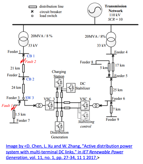
As is shown in the distribution network
- Back-to-back converter as a controllable voltage/current source between Feeder 3 and 6.
- This means that the power flow within the network can be re-distributed in a continuous manner.
- Since the converters’ fault currents to the AC side are controllable with the power converter, it does not need to change the established protection system.
- The undesirable loading conditions against DG can be instantly adjusted to enable more DG connection in the network
Increasing the Hosting Capacity - 4
- Prioritizing Renewable Energy
● When the hosting capacity has to be shared between different generators, priority could be given to the most environment-friendly sources of energy
- Dynamic loadability
● A real-time detection is placed on the ambient temperature and wind speed of the targeting feeders
● Higher feeder loading should be allowed when the wind speed is high or the temperature is low as a better cooling condition can raise up the practical thermal limit of a feeder
For further reading about this unit, please read:
Chapter 4.5 , Math Bollen And Fainan Hassan - Integration of Distributed Generation in the Power System
Chapter 7, Jenkins, N., etc. “Distributed Generation”