Wk 1
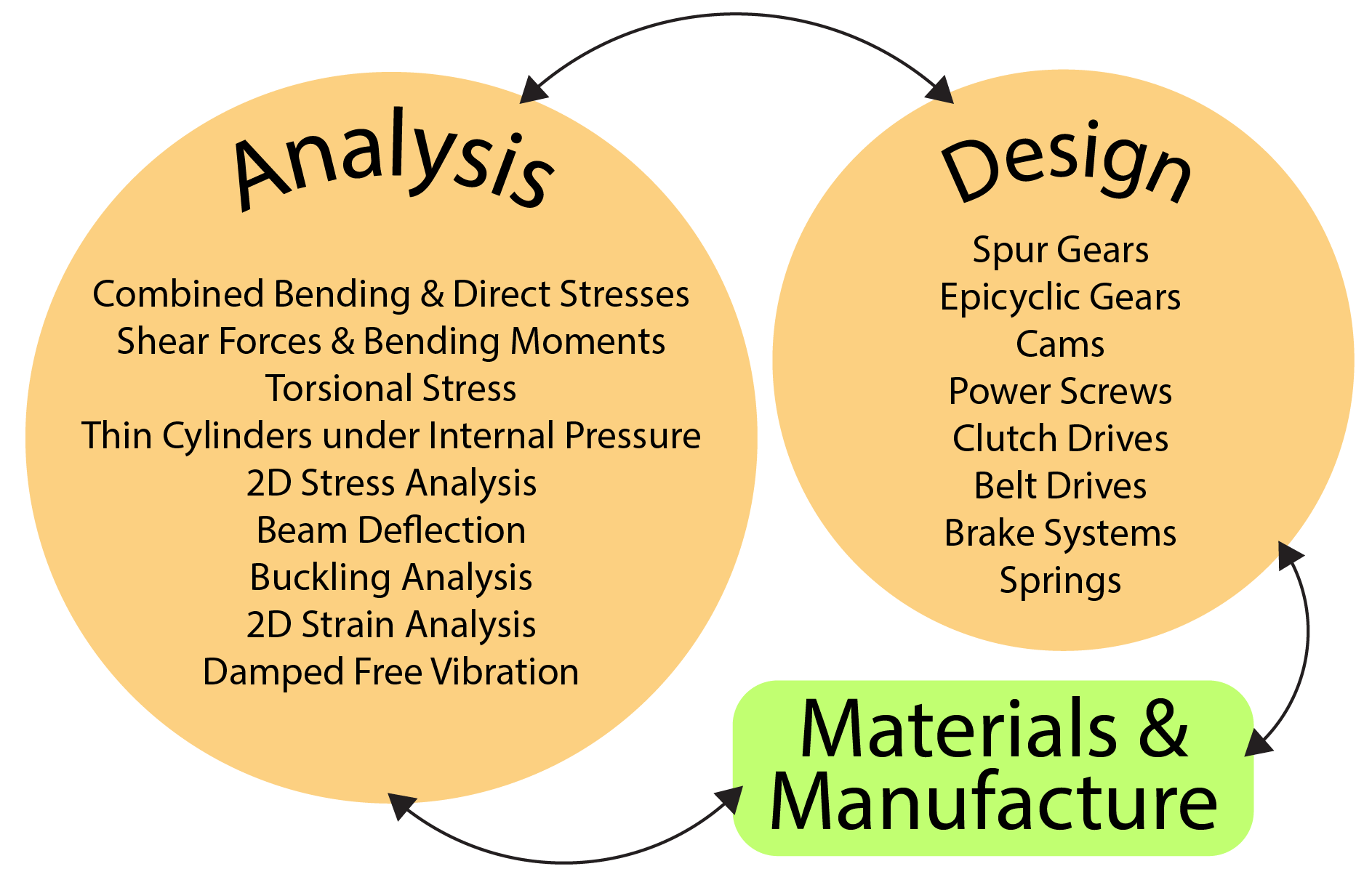
- So, all engineers need some background in Engineering Design & Analysis to apply to the design and analysis of components!
 Click to replay above animation
 Click to Enlarge Diagram
Direct and Bending Stresses:
Statics: Stress, Strain and Elastic Behaviour- Stress, Strain and Elastic Behaviour
- Direct Stress
- Direct Strain
- Elastic Material
- Poisson’s Ratio
- Shear Stress
Introduction
- All of the engineering photographic examples shown in the right-hand corner of the page require the application of the principles of mechanical engineering, combined with:
– Analysis:Forces, Stresses, Displacements, Motion and Vibration– Design:Shape, Form and Materials– Components:Gears, Springs, Cams and Linkages– Manufacture:Processes, Methods and Production– Computer Applications :Software , Hardware, Data and Communication– Electrical Power– Electronics
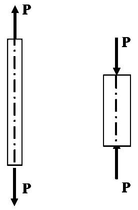
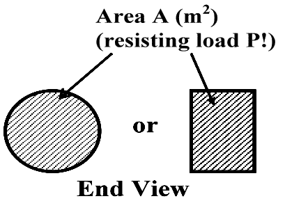
Direct Stress
Direct stress can be tensile (+ve) or compressive (-ve) and can be calculated using Eqn.(1):
 $$ \large σ = \frac{P}{A}
(N/m^2)
. $$
‘Tie’ (+ve Stress) ‘Strut’, ‘Column’, ‘Pillar’ (-ve Stress)
$$ \large σ = \frac{P}{A}
(N/m^2)
. $$
‘Tie’ (+ve Stress) ‘Strut’, ‘Column’, ‘Pillar’ (-ve Stress)
- Note: take care with compression loading - for longer, thinner structures/components, ‘buckling’ could occur ! – more later!
Statics: Stress, Strain and Elastic Behaviour
- 📷 Effects of loading on components/structures can be seen here
Stress
- Externally applied loads produce internal ‘reaction’ forces within a body if the body is solid. These internal forces resist deformation.
The ratio of these forces to the area on which they are applied is called Stress.
- EQN 1
$$ stress = \frac{load (N)}{Area(m^2)} \quad \textit{e.g.} \quad σ = \frac{P}{A} (N/m^2) . $$
- Note: Units:
1 N/m
1 MN/m $ ^2 $ = 1 N/mm $ ^2 $
Elastic Material
- An elastic material returns to its original shape and dimensions when an externally applied load is removed. The material obeys Hooke’s Law which states that displacement varies directly with load, and hence, $$ Stress \; \alpha \; Strain, \quad \textit{i.e.}\quad \frac{Stress}{Strain}= constant. $$
The constant is termed Young’s Modulus of Elasticity E and has the units N/m$ ^2$ $\textit{i.e.}$,
- EQN 3
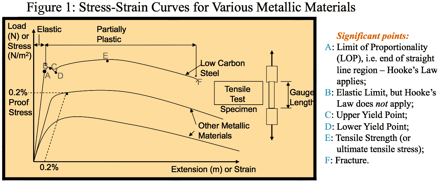
$$ \large E = \frac{\sigma}{\epsilon} (N/m^2) . $$ A value for E for a material can be obtained from a tensile test where a test specimen of the material of specified shape and dimensions is stretched until it breaks. E is calculated as the gradient of the straight line within the elastic behaviour region of the stress-strain graph obtained from the test.
- 📷 Figure 1 - which can be seen here shows typical tensile test curves for various materials with significant points highlighted.
- Note: Only low carbon steel shows an upper and lower yield point, with most other metallic materials displaying a smooth transition from elastic behaviour to plastic deformation. For a comparison of material strength, a proof stress is normally measured from the stress-strain curve at a particular percentage strain, $\textit{i.e.}$ 0.2% is commonly used and is highlighted in the graph above.
Statics: Stress, Strain and Elastic Behaviour
Direct Strain
- The basic definition of strain is the ratio of change in dimension to the original dimension.
A component subjected to direct stress will change in length, with an increase in length (+ve) for tensile loading and a decrease (-ve) in length for compressive loading.
- 📷 The ratio of the change in length to the original length is termed Strain and is non-dimensional - click to view
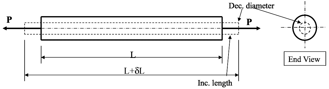
More specifically, with regards to a components length, a strain along the length is termed the LONGITUDINAL STRAIN $ \epsilon _L $ and is defined by Eqn.(2).
- EQN 2
$$ strain = \frac{ChangeinLength(mm)}{OriginalLength(mm)} \quad \textit{e.g.} \quad \epsilon _L = \frac{\delta L}{L} . $$
- 📷 Longitudinal Strain Illustrated Here - click to view
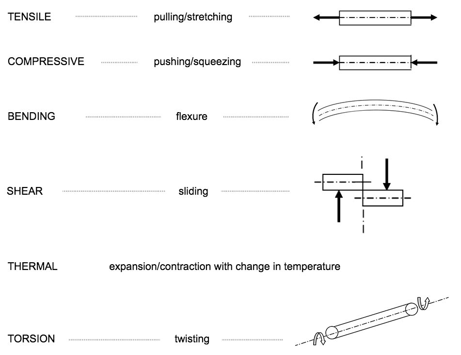
 TENSILEpulling/stretching
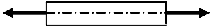 COMPRESSIVEpushing/squeezing
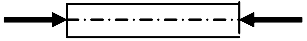 BENDINGflexure
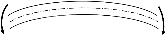 SHEARsliding
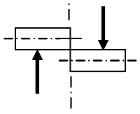 THERMALexpansion/contraction with change in temperatureo
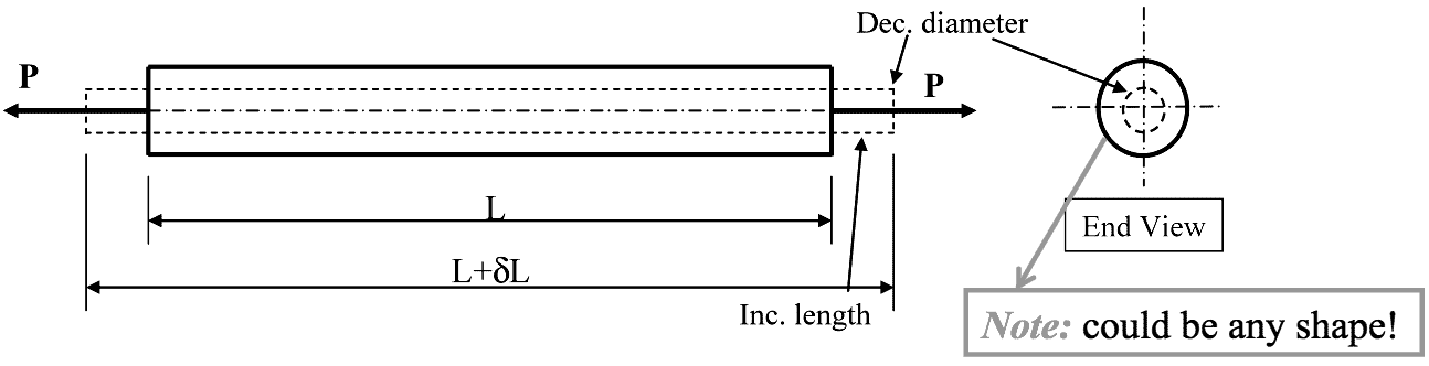

Elastic Material
- The lateral strain is defined as the ratio of change in dimension to original dimension where the dimension relates to the cross-section (e.g. radius, diameter, width, depth etc), $\textit{i.e.}$
EQN 4$$ strain = \frac{ChangeinLength(mm)}{OriginalLength(mm)} \quad \textit{i.e.} \quad \epsilon _{Lat} = \frac{\delta R}{R} $$- Finally, the ratio of the lateral strain to the longitudinal strain is defined as Poisson's Ratio denoted ν, $\textit{i.e.}$
EQN 5$$ Poisson’s \; Ratio = \frac{LateralStrain}{LongitudinalStrain} \quad \textit{i.e.} \quad v = \frac{\epsilon _{Lat}}{\epsilon _{L}} $$- Note: For most metallic materials, 0.25 < ν < 0.33.
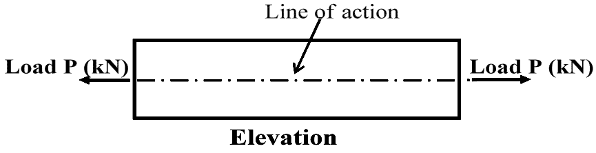
Shear Stress
- Shear stress occurs when a component is subjected to forces where the ‘lines of action’ act at a distance apart causing a ‘sliding’ action to occur and the creation of a shear plane as shown in the figure below. These shear forces set-up shear stress (denoted $ \tau $) in the material which acts in a direction tangential to the area on which the shear stress acts.
EQN 6$$ shear stress = \frac{ShearForce}{ShearArea} \quad \textit{i.e.} \quad \tau = \frac{Q}{A} (N/m^2) $$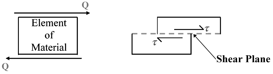
- ⬇ Download worked example
Statics: Stress, Strain and Elastic Behaviour
Poisson’s Ratio
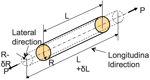
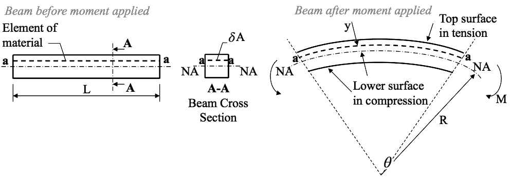
- When a component is subject to a direct load (tensile or compressive) which sets-up a direct stress and hence a direct strain, strain will occur not only along the component length (longitudinal), it will also occur across the cross-section, i.e. lateral strain. Hence changes in both component length and cross-section dimensions take place. This is highlighted by Figure 20 which shows a round bar of radius R and length L subjected to a direct tensile load P causing it to extend in length by $ \delta $L and reduce in radius by $ \delta $R. Hence, as previously discussed, the longitudinal strain is defined as the ratio of change in length to the original length, $\textit{i.e.}$
$$ \huge \epsilon _L = \frac{\delta L}{L} $$
TENSILEpulling/stretchingCOMPRESSIVEpushing/squeezingBENDINGflexureSHEARslidingTHERMALexpansion/contraction with change in temperatureo- The lateral strain is defined as the ratio of change in dimension to original dimension where the dimension relates to the cross-section (e.g. radius, diameter, width, depth etc), $\textit{i.e.}$
- The Section Properties: Centroids and 2nd Moment of Area
2$ ^{nd} $ Moments of Area
From earlier work, a moment was defined as a force $ x $ (perpendicular) distance. From above, a 1$ ^{st} $ moment of area was defined as area $ x $ distance to centroid. Hence, 2$ ^{nd} $ moment of area is defined as the 1st moment of area $ x $ distance to centroid. Consider the rectangular section shown, which has width $ b $ and depth $ d $.
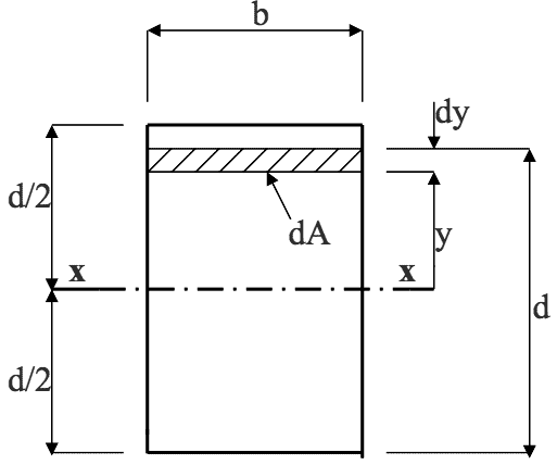 Axis $ x-x $ is the horizontal centroidal (neutral) axis.
Area of shaded element $ = dA = b.dy$
$ 1^{st} $ moment of elemental area about x-x axis = y.dA (since dy is very small)
$ 2^{nd} $ moment of elemental area $ = y.(y.dA) = y^2.dA $
The 2$ ^{nd} $ moment of the whole area about x-x is obtained by integrating (i.e. summation) each elemental area, and is usually denoted by I, $\textit{i.e.}$$$ I_{xx} = \int y^2 .dA = \int\limits_{-d/2}^{+d/2} b.y^2 .dy = b. \begin{bmatrix}\frac{y^3}{3}\end{bmatrix}^{+d/2} _{-d/2} $$ $$ = \frac{b}{3}. \begin{bmatrix}\frac{d^3}{8} - \bigg( - \frac{d^3}{8} \bigg)\end{bmatrix}=\frac{b}{3} . \begin{bmatrix}\frac{d^3}{4}\end{bmatrix} $$- Hence, for a rectangle, the 2$ ^{nd} $ moment of area about the x-x centroidal axis is given by:
EQN 8$$ I_{xx} = \frac{bd^3}{12} $$
Statics: Stress, Strain and Elastic Behaviour
Bending Stresses
- Section Properties: Centroids and 2$ ^{nd} $ Moment of Area
- 📷 1$ ^{st} $ Moments of Area For the common cross-sections, seen at this link , the neutral axes coordinates $ \overline{x} $ and $ \overline{y} $ are found by inspection or from simple formulae. However, for more complex geometry, the position of the centroid and hence the neutral axes is found by considering $ 1^{st} $ moments of area. A $ 1^{st} $ moment of area is defined as area $\textbf{x}$ distance from a reference point to the area centre, $\textit{i.e.}$
EQN 7$$ \huge \Sigma \normalsize A \overline{x} ^{=} \huge \Sigma \normalsize 1^{st} \textit{moments} ^{=} \huge \Sigma \normalsize Ax $$
$$ \textit{or} \quad \overline{x} = \frac{\huge \Sigma \Large ^{A.x}}{\huge \Sigma \Large ^{A}} \quad \textit{and} \quad \overline{y} \frac{\huge \Sigma \Large ^{A.y}}{\huge \Sigma \Large ^{A}} . $$ where A = elemental area, and $ \textit{x} $ and $ \textit{y} $ are distances from a reference point to the centre of elemental area.
- Section Properties: Centroids and 2nd Moment of Area
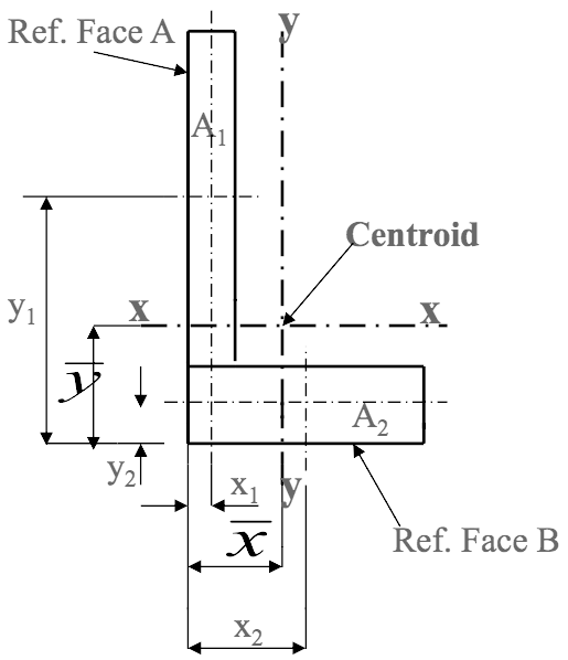
From Ref. above Face A:$$ \overline{x} = \frac{\huge \Sigma \Large ^{A.x}}{\huge \Sigma \Large ^{A}} = \quad \frac{A_1.x_1 + A_2.x_2}{A_1 + A_2} $$From Ref. above Face B:$$ \overline{y} = \frac{\huge \Sigma \Large ^{A.y}}{\huge \Sigma \Large ^{A}} = \quad \frac{A_1.y_1 + A_2.y_2}{A_1 + A_2} $$ 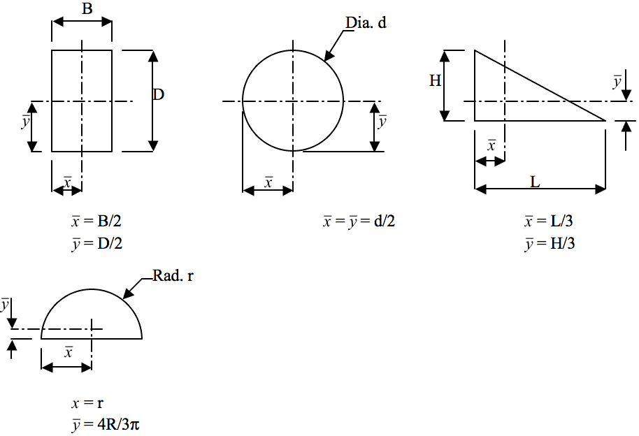
- The Section Properties: Centroids and 2nd Moment of Area
- The Section Properties: Centroids and 2$ ^{nd} $ Moment of Area
2$ ^{nd} $ Moments of Area
Consider the circular section shown which has a diameter d and an outside radius $ R $.
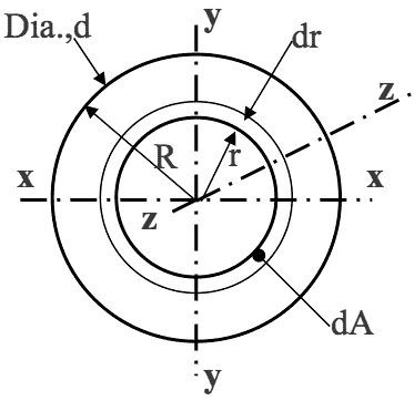 For circle, elemental area = dA = 2$ \pi $ r.dr
$ 1^{st} $ moment of area about z-z axis = r.dA (since dr is very small)
$ 2^{nd} $ moment of area about z-z axis = r$ ^2 $.dA
Hence for whole area:$$ I_{zz} = \int\limits_{0}^{R} r^2 .dA = 2\pi \int\limits_{0}^{R} r^3 .dr = 2\pi. \begin{bmatrix}\frac{r^4}{4}\end{bmatrix}^{R} _{0} $$ $$ = \frac{\pi R^4}{2} =\frac{\pi d^4}{32} $$
Now,
$ \quad \large I_{zz} = I_{xx} $ + $ \large I_{yy} $ where $ \large I_{xx} = I_{yy} $ for a circle, $ \large I_{xx} = I_{yy} = \frac{I_{zz}}{2}$EQN 10$\textit{i.e.}$$$ I_{xx} = I_{yy} \frac{\pi d^4}{64} $$
Statics: Stress, Strain and Elastic Behaviour
Bending Stresses (cont.)
- Section Properties: Centroids and 2$ ^{nd} $ Moment of Area
$ 2^{nd} $ Moments of Area
Similar to the definitions and calculations for $ I_{xx}, I_{yy} $ can be calculated for the above rectangle as follows: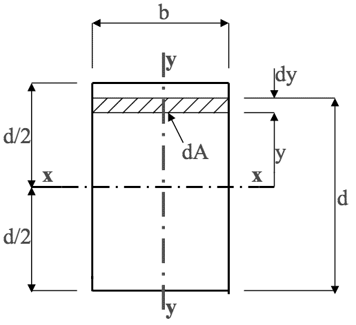
$$ I_{yy} = \int x^2 .dA = \int\limits_{-b/2}^{+b/2} d.x^2 .dx = d. \begin{bmatrix}\frac{x^3}{3}\end{bmatrix}^{+b/2} _{-b/2} $$ $$ = \frac{d}{3}. \begin{bmatrix}\frac{b^3}{8} - \bigg( - \frac{b^3}{8} \bigg)\end{bmatrix}=\frac{d}{3} . \begin{bmatrix}\frac{b^3}{4}\end{bmatrix} $$EQN 9$\textit{i.e.}$$$ I_{yy} = \frac{db^3}{12} $$where, in Eqns.(8,9), b = width and d = depth.
[Note: the units for I are in mm$^4 $ or m$^4 $.] TENSILEpulling/stretchingCOMPRESSIVEpushing/squeezingBENDINGflexureSHEARslidingTHERMALexpansion/contraction with change in temperatureo- The Section Properties: Centroids and 2$ ^{nd} $ Moment of Area
- The Section Properties: Centroids and 2$ ^{nd} $ Moment of Area
2$ ^{nd} $ Moments of Area for Common Sections
Consider the hollow circular section shown below
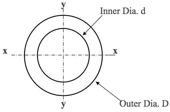 $$
I_{xx} = I_{yy} = \frac{\pi}{64} (D^4 - d^4)
$$
$$
I_{xx} = I_{yy} = \frac{\pi}{64} (D^4 - d^4)
$$
- 2$ ^{nd} $ Moments of Area: Parallel Axis Theorem
For common or standard cross-sections like rectangles and circles, calculation of the $ 2^{nd} $ moment of area is straight forward using Eqns.(8) and (10). However for unsymmetrical shapes like ‘T’, ‘L’ and ‘C’ sections, use has to be made of the Parallel Axis Theorem. Consider the simple example shown used to demonstrate parallel axis theorem.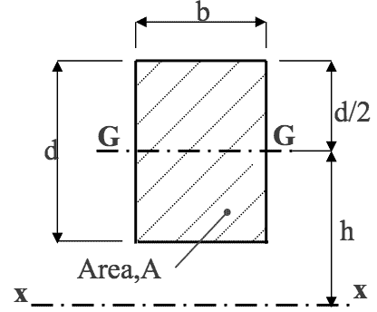
For the rectangle, $ I_{GG} $ can be easily calculated by applying Eqn.(8), i.e. $$ I_{GG} = \frac{bd^3}{12} $$
The $ 2^{nd} $ moment of area of the whole cross-section about the parallel axis x-x I$ _{xx} $, can be obtained using Eqn.(12).- EQN 12
$$ I_{xx} = I_{GG} + Ah^2 $$ where, A = cross-sectional area (mm$ ^2 $)
and h = distance between the two parallel axes (mm).
Statics: Stress, Strain and Elastic Behaviour
Bending Stresses (cont.)
- Section Properties: Centroids and 2$ ^{nd} $ Moment of Area
2$ ^{nd} $ Moments of Area for Common Sections
The 2$ ^{nd} $ moment of area of commonly used cross-sections which comprise of standard rectangular and circular sections can be easily found by adding or subtracting the appropriate I value as required. Consider the ‘I’ shape section shown.
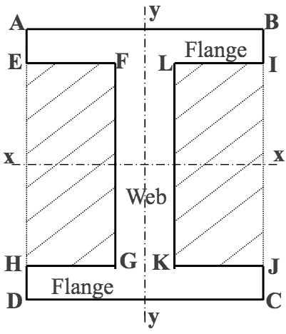
The $ 2^{nd} $ moment of area for the ‘I’ section shown is found as follows:
$$ I_{xx} = \begin{bmatrix}I_{xx}\end{bmatrix} \tiny ABCD \normalsize - 2 \begin{bmatrix}I_{xx}\end{bmatrix} \tiny EFGH $$ $\textit{i.e.}$ $$ (Outer) \\ I_{xx} = \begin{bmatrix}bd^3/12\end{bmatrix} \tiny ABCD \normalsize $$
$$ (Shaded) \\ - 2 \begin{bmatrix}bd^3/12\end{bmatrix} \tiny EFGH $$ Also $$ I_{yy} = 2\begin{bmatrix}bd^3/12\end{bmatrix} \tiny ABIE \normalsize + \begin{bmatrix}bd^3/12\end{bmatrix} \tiny FLKG $$ TENSILEpulling/stretchingCOMPRESSIVEpushing/squeezingBENDINGflexureSHEARslidingTHERMALexpansion/contraction with change in temperatureo- The Section Properties: Centroids and 2$ ^{nd} $ Moment of Area
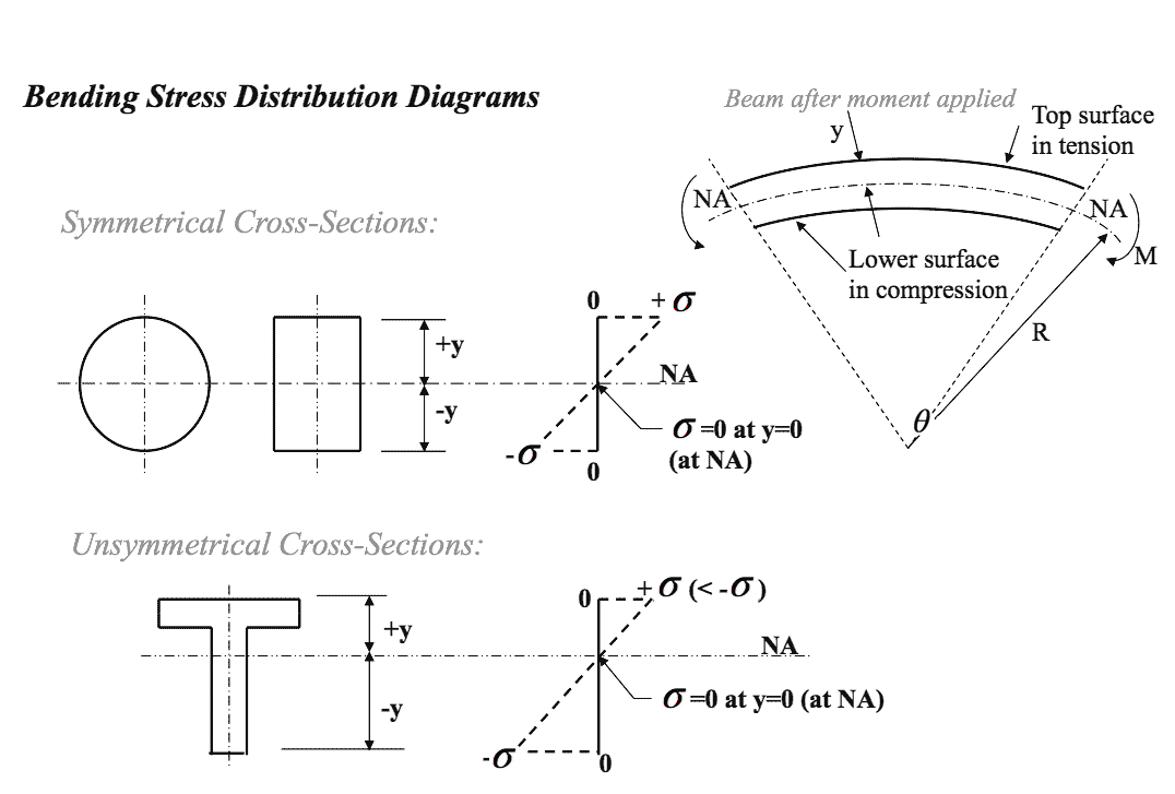
Bending Stress Distribution Diagrams From the theory of bending equation given by Eqn.(4), it can be seen that the magnitude of the bending stress $ \sigma $ for a particular cross-section subjected to a bending moment $ M $, and with a 2$ ^{nd} $ moment of area $ I $, varies through the cross-section and is dependent upon the value of $ y , \textit{i.e.}$
$$ \frac{M}{I} = \frac{\sigma}{y} = \frac{E}{R} $$ $ \textit{i.e.}$ $$ \sigma = \frac{My}{I} $$- Note: Refer to diagram on the left collumn of the page.
- 📷 Bending Stress Distribution Diagrams.
- ⬇ Download worked example
Statics: Stress, Strain and Elastic Behaviour
Bending Stresses (cont.)
- When a bending moment is applied to a beam it will bend as shown.
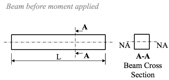 The upper surface becomes extended
and in tension and the lower surface
becomes compressed and in compression.
The upper surface becomes extended
and in tension and the lower surface
becomes compressed and in compression.
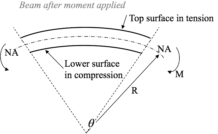 If the top surface is in tension which
leads to a +ve tensile stress and the
lower surface is in compression which
leads to a -ve compressive stress.
If the top surface is in tension which
leads to a +ve tensile stress and the
lower surface is in compression which
leads to a -ve compressive stress.
- 📷 Beam After Moment Applied - Diagram Seen Here.
Equations (1) and (2), seen in earlier tabs, are generally combined and written as follows:- EQN 4
$$ \frac{M}{I} = \frac{\sigma}{y} = \frac{E}{R} $$ This is the general bending equation and is an exact solution for the case of pure bending for elastic behaviour where the stress is limited to the stress at the limit of proportionality for the material.
Statics: Stress, Strain and Elastic Behaviour
Summary
- ⬇ Bending DirectStress Summary
$ \quad \large \sigma = \frac{My}{I} \quad $ [+ve – tensile stress; -ve – compressive stress]
$ \large \epsilon _L = \frac{\delta L}{L} \quad $ [Strain along the length of a component - longitudinal]
$ \large E = \frac{\sigma}{\epsilon} (N/m^2) \quad $ [Young’s Modulus of Elasticity for material]
$ \large \epsilon _{Lat} = \frac{\delta R}{R} \quad $ [Strain along the radius of a component - lateral]
$ \large v = \frac{\epsilon _{Lat}}{\epsilon _{L}} \quad $ [Poisson's Ratio for material]
$ \large \tau = \frac{Q}{A} \quad $ [Shear stress]
$ \large \frac{M}{I} = \frac{\sigma}{y} = \frac{E}{R} \quad $[Theory of Elastic Bending]