Week 11: Engineering Design & Analysis 2

Wk 11

Clutch Drive System Design

Definition

Plate Clutches
– Constant Pressure

– Constant Wear

Cone Clutches
– Constant Pressure

– Constant Wear

Worked Examples

Belt Drive System Design

Introduction

Power Transmission

Crossed Belt Drives

Ratio of Belt Tensions

Centrifugal Tension

Belt Speed for Maximum Power Transmission

Initial Belt Tension

Vee-Belt Drives

Worked Examples
(cont.)
Uniform Pressure:

$ W = \pi . p \bigg( r_1^2 - r_2^2 \bigg) \therefore p = \frac{W}{\large \pi ( r_1^2 - r_2^2 )} $

and:
$ T = \frac{2}{3}\pi . \mu .p ( r_1^3 - r_2^3 ) $

Finally:
$ T = \frac{2}{3} . \mu . W \frac{(\large r_1^3 - r_2^3 )}{(\large r_1^2 - r_2^2 )} $

Uniform Wear:
$ W = 2 \pi . \int\limits_{r_2}^{r_1} p .r .dr = 2 \pi . p .r . \int\limits_{r_2}^{r_1} dr $
$ = 2 \pi . c \int\limits_{r_2}^{r_1} dr = 2 \pi . c (r_1 - r_2)$

Therefore:
$ T = 2 \pi \mu . \int\limits_{r_2}^{r_1} p .r^2 .dr \; \Rightarrow T = 2 \pi \mu . p r \int\limits_{r_2}^{r_1} r .dr $
and:
$ \Rightarrow T = 2 \pi \mu . c \int\limits_{r_2}^{r_1} r .dr = \mu W \frac{r_1 + r_2}{2}$
Finally:
$ \Rightarrow T = \mu WR \quad Eqn \; (3.2) $

Application of Equations
– Uniform Pressure – new clutch

– Uniform Wear – worn clutch

Definition

A clutch is a friction device designed to permit the connection and disconnection of power transmission shafts.
Figure 3.1 shows a typical single plate clutch schematic arrangement where the inner plate is free to slide on axial splines cut in a hub keyed to the driving shaft. The outer plate is free to slide axially in splines cut in a housing keyed to the driven shaft. The axial force exerted on the plates by a toggle mechanism is transmitted through each plate.

Figure 3.1

Two plates held in contact by axial thrust force ‘W’:
$ \text{– Normal force on elementary ring} = p.2πr.dr $

$ \text{– Total axial force,} W = 2 \pi. \int\limits_{\large r_2}^{\large r_1} p .r .dr $

$ \text{– Friction force on elementary ring} = \mu .p.2 \pi r.dr $

And, Moment of friction force about the axis $ = \mu .p.2 \pi r.dr $

Torque Transmitted: $ \text{Torque transmitted,} T = 2 \pi \mu \int\limits_{r_2}^{r_1} p .r^2 .dr $

Multiple Plate Clutch
• Figure 3.2: A typical multi-plate clutch arrangement.
(Cont.)

Total friction drag on ring $ \normalsize = \mu . p . 2 \pi . r . \large \frac{dr}{sin \; \beta} \small \; (= \mu \; x \; \text{normal force)} $

∴ Moment of force about axis $ \normalsize = \mu . p . 2 \pi . r^2 . \large \frac{dr}{sin \; \beta} $

∴ Torque transmitted, $ T \normalsize = \large \frac{2 \pi \mu}{sin \; \beta} \normalsize . \int\limits_{r_2}^{r_1} p . r^2 . dr $

Uniform Pressure
$ \normalsize T = \large \frac{2}{3} . \frac{\mu . W}{sin \; \beta} \frac{(r_1^3 - r_2^3 )}{((r_1^2 - r_2^2 ))} \normalsize $

Uniform Wear
$ T = \large \frac{\mu.W}{2 sin \; \beta} \normalsize (r_1 + r_2)$

Or
$ T = \large \frac{\mu.W R}{sin \; \beta} \normalsize \; $

⬇ Clutches Worked Example

Cone Clutches

📷 A cone clutch diagram - seen here larger

Normal force on elementary ring
$ \normalsize = p.2 \pi .r . \large \frac{dr}{sin \; \beta} $

Axial component of normal force
$ \normalsize = p.2 \pi .r . \large \frac{dr}{sin \; \beta} \normalsize . sin \; \beta = 2 \pi . p . r .dr $

∴ Total axial force,
$ W = 2 \pi . \int\limits_{r_2}^{r_1} p .r .dr $

Figure 3.3: A typical cone clutch.
Power Transmission
F₁ = the ‘tight side’ tension

F₂ = the ‘slack side’ tension

Pulley drives the belt in a clockwise direction, and assuming no slip linear speed of belt is equal to peripheral speed of pulley

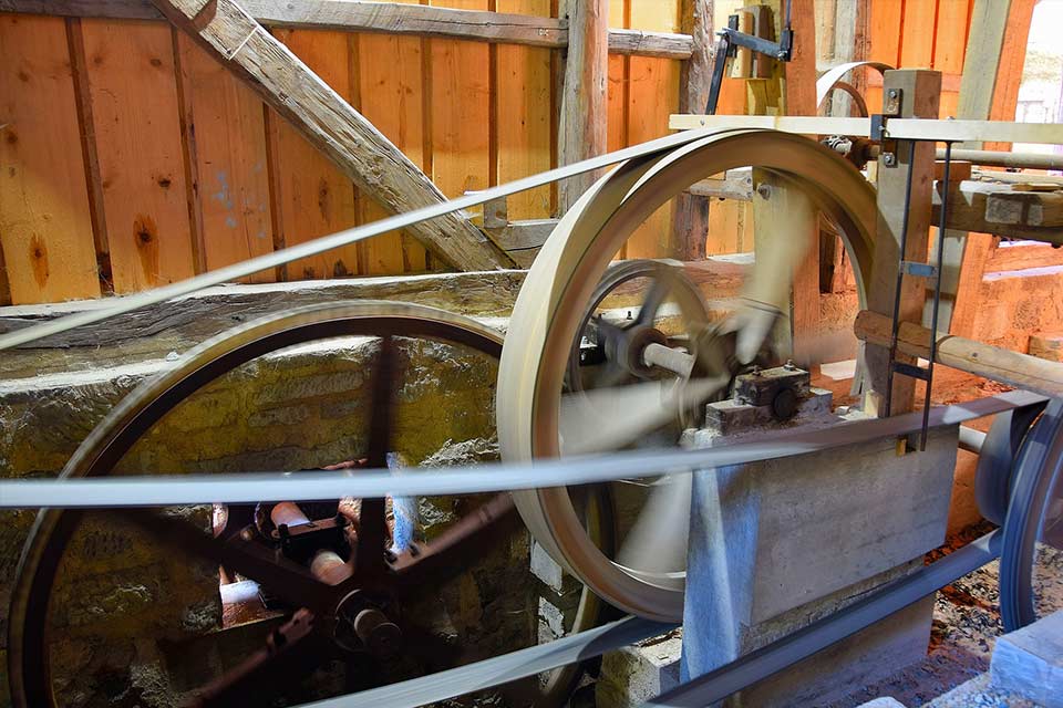
Belt Drive System Design

Introduction

📷 Types of Belt
– Flat belt

– Vee-type belt

Advantages
– Quiet running

– Clean and easy to maintain

– Relatively economical

Features
– Continuous belt

– Pulleys keyed to shaft

– Frictional contact between belt and pulley

Belt Drives - Introduction
Power may be transmitted by means of a belt drive (either flat or vee-type) with the main advantages gained in using them including quiet running, clean and easy to maintain, and relatively economical. The belt is continuous and passes over pulleys which are keyed to shafts. The effectiveness of a belt drive depends upon friction between the belt and the pulley, and on the angle of contact between the belt and the pulley surface. Before belt drives now are considered in detail, consider Figure 4.1:

Figure 4.1: A typical multi-plate clutch arrangement.
Crossed Belt Drive

Ratio of Belt Tensions

Power transmitted depends on F₁ – F₂

For a higher ratio of F₁ / F₂ more power will be transmitted
– However there is a limiting ratio at which the belt will slip on the pulley:

– Ratio of F₁ / F₂ depends on:

the coefficient of friction (μ) between the belt and the pulley;

the angle of lap (θ) of the belt round the pulley, and that an increase in either μ and θ will lead to an increase in the ratio (F₁/F₂)

It can be shown that the limiting ratio of tensions (F₁/F₂) is given by: $ \large \frac{F_1}{F_2} \normalsize = e ^{\mu \theta} $

Angle of Lap

Power Transmission (Cont.)

Net clockwise torque on the pulley
T = F₁.r – F₂.r = (F₁ – F₂)r

Now, Power
P = Tω ∴ P = (F₁ – F₂)rω

The difference in tensions (F₁ – F₂) is referred to as the effective tangential force.

Also, note that since v = ωr, then:
P = (F₁ – F₂)v (W)

Angle of Lap
θ represents the angle of lap, i.e. angle of contact between belt and pulley.
Belt Speed for Maximum Power Transmission

Power transmitted:
(F₁ – F₂)v = [(F₁ – F_C) - (F₂ – F_C)]v

From previous:
$ F_2 - F_c = \large \frac{F_1 - F_c}{e ^{\mu \theta}} $

Therefore, power transmitted:
$ (F_1 - F_c) (1 - \frac{\large 1}{e ^{\large \mu \theta}} ) v = k (F_1 - mv^2) v \; \; Eqn \; (4.5) $

Where:
$ k = constant = 1 - \frac{\large 1}{e ^{\large \mu \theta}} $

For maximum power, differentiate with respect to velocity and equate to 0:
$ \frac{\large d [( F_1 - mv ^2)v]}{\large dv} = 0 $

Hence, F₁ – 3mv² = 0

Therefore, F_C = F₁/3 (N)

The maximum power is then obtained by substituting this value of F_C and the corresponding value of $ v $ in Eqn 4.5 above.

During start-up, no centrifugal effects are present and therefore power transmitted will be different from that under normal conditions

Initial Belt Tension

Initial tension in belt is F₀

Once running:

– The tension in the tight side increases from F₀ to F₁ and

– On the slack side decreases from F₀ to F₂

Assuming Hooke’s law is obeyed and the length remains constant:
F₁ – F₀ = F₀ – F₂ and
F₁ + F₂ = 2F₀

Centrifugal Tension

Belt has mass per unit length (m)

F_c is the centrifugal tension

Centrifugal force acting on an element of belt:
$ F = 2.F_c.sin \frac{\large d \theta}{\large 2} =2 . F _c. \frac{\large d \theta}{\large 2} $

Mass of belt section $ = m.r.d \theta $

Centrifugal force = mv²/r

Therefore:
$ (m.r.d \theta) \frac{\large v^2}{\large r} = F_c. d \theta $
$ \Rightarrow F_c = mv^2 $

θ represents the angle of lap, i.e. angle of contact between belt and pulley.

Allowance for Centrifugal Tension
$ \large \frac{F_1 - F_c}{F_2 - F_c} = e ^{\mu \theta} $

F₁ – F_C and F₂ – F_C are the effective driving tensions

Vee Belts

The belt tension sets up a radial force R acting towards the centre of the pulley
$$ sin \; \alpha = \frac{R/2}{R_N} \quad \quad \frac{R}{2} = R_N \; sin \; \alpha $$ therefore:
$$ R = 2R_N \; sin \; \alpha \quad \quad 2R_N = \frac{R}{sin \; \alpha} $$

Now, for flat belts, the friction force = μR (see above)

And for vee-belts, the friction force = 2μR_N (two friction surfaces) =
$$ \frac{\mu R}{sin \; \alpha} $$

Hence, the belt tension formula for flat belts is modified for vee-belts and becomes:
$$ \frac{F_1}{F_2} = e ^{\frac{\Large \mu \theta}{\Large sin \; \alpha}} $$

⬇ Belt Drive Worked Example

Hinged Ends - L_f /D	Hinged Ends - K_L	Built-in-Ends - L_f /D	Built-in-Ends - K_L
1	0.72	1	0.72
2	0.63	2	0.71
3	0.38	3	0.68
4	0.20	4	0.63
5	0.11	5	0.53
6	0.07	6	0.38
7	0.05	7	0.26
8	0.04	8	0.19

Note: A further measure that can be taken to avoid buckling, is to ensure that the spring index C is as large as possible.

Summaries

⬇ Clutches and Belt Drives Summary

Clutches

📷 Nomenclature for Clutches

Flat Belt Summary

Main factors governing difference in tensions

– Angle of Lap

Pulley Diameters

Pulley Centre Distance

– Coefficient of Friction

Limited by requirement for smooth pulley surface

Can use a semi-liquid preservative compound to increase friction

Vee Belt Summary

Typical groove angle around 40⁰

Belt should not contact the bottom of the groove

Same design procedure as flat belts

– Pulley centre distance

– Belt tensions

– Power transmitted

Belt cross-sectional area

Number of belts required

Symbol	Description	Unit
A	Contact area	m²
dr	Small portion of contact disc	m
n	Number of contact pairs (plate clutch)	-
p	Intensity of pressure between contact surfaces	Nm^-2
R	Mean radius	m
r₁	Outer radius	m
r₂	Inner radius	m
T	Transmitted torque	Nm
W	Axial thrust force	N

β	Cone angle	degrees
μ	Coefficient of friction	-

Tutorials

⬇ Clutches Tutorial

⬇ Belt Drives Tutorial