Wk 3
-

Laplace Transforms: the $s$ domain
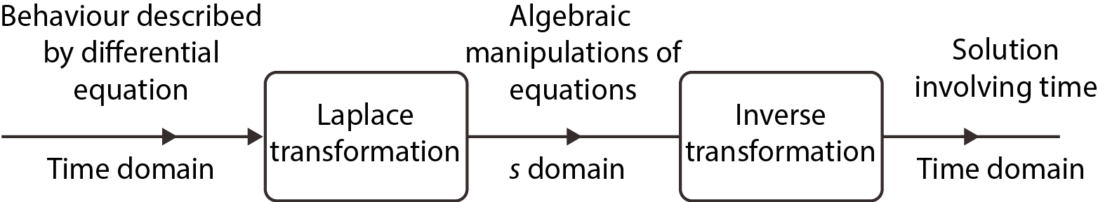
- The Laplace transform is a method of transforming differential equations into more easily solved algebraic equations. Differential equations which describe how a circuit or component behave with time are transformed into simple algebraic relationships, not involving time, where we can carry out normal manipulation ( add, subtract, multiply and divide ) of the quantities.
Reading for Week 3
GCU Control Engineering 3 lecture notes, Part I, Chapter 3.Control Systems: Appendix B
Further reading:
Introduction to Linear Control Systems: Appendix A2-A2.2;
Additional questions that you should attempt:
GCU Control Engineering 3 lecture notes, Part II, Chapter 16Control Systems: Chapter 3, Problems 1 to 14Links:
We talk of the circuit / component or system behaviour in the time domain ($t$) being transformed into the $S$ ( or Laplace ) domain, in which the algebraic manipulations can be carried out. Then we use an inverse transform describing how the signal varies in time, i.e. transform from the s-domain back to the time domain.
Figure 3.1 (click the link below) describes the Laplace transform process. The tables on tab 3.1 and 3.2 are a list of differential equations in the time domain and their equivalent Laplace transformations in the $s$- domain.
📷 Figure 3.1 - The Laplace Transform Process
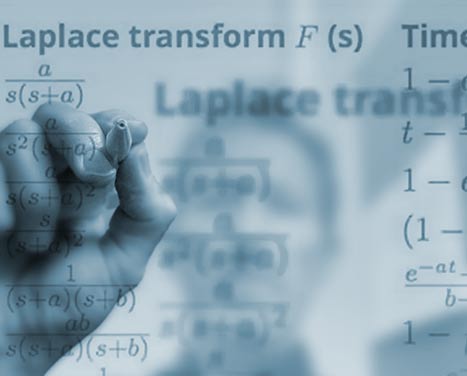
Table of Laplace transforms
For simple functions, it is straightforward to calculate Laplace transforms using integration by parts. However, there are a number of forms that arise repeatedly and it is more convenient to use a table of transforms to solve these, rather than calculating each transform manually (seen on tab 3.1 and 3.2).
Note: some of the images shown in the tabbed pages can be enlarged by clicking on them.

- The Laplace transform is a method of transforming differential equations into more easily solved algebraic equations. Differential equations which describe how a circuit or component behave with time are transformed into simple algebraic relationships, not involving time, where we can carry out normal manipulation ( add, subtract, multiply and divide ) of the quantities.
Laplace Transforms
- A list of differential equations in the time domain and their equivalent Laplace transformations in the $s$- domain
\begin{align*} \textbf{Laplace transform $F$ (s)} && \textbf{Time function $f$ (t)} && \textbf{Desciption of time function} \\ \\ \frac{a}{s} && a && \text{constant, i.e. $a$=1, $a$=2, etc.} \\ a F(s) && a f(t) && \text{constant x equation} \\ s F (s) && \frac{d}{dt} f (t) && \text{first order differentiation} \\ s^n F (s) && \frac{d^n}{dt^n} f (t) && \text{'n' th order of differentiation e.g.} n = 2 \frac{d^2 f (t)}{dt^2} \\ \frac{1}{s} F (s) && \int_{0}^{t} f (t) dt && \text{Integration} \\ 1&& && \text{unit impluse} \\ %Figure *** f(t) against t \frac{1}{s} && && \text{unit step function} \\ %Figure *** f(t) against t \frac{e^{-ST}}{s} && && \text{delayed unit step function} \\ %Figure *** f(t) against t \frac{1 - e^{-ST}}{s} && && \text{recangular pulse of duration T} \\ %Figure *** f(t) against t \frac{1}{s^2} && t && \text{unit slope ramp input function} \\ %Figure *** f(t) against t \frac{1}{s^3} &&\frac{t^2}{2} && \\ \frac{1}{s + a} && e^{-at} && \text{exponential decay} \\ %Figure *** f(t) against t \frac{1}{(s + a)^2} && t e^{-at} && \\ \frac{2}{(s + a)^3} && t^2 e^{-at} && \\ \end{align*}
- A list of differential equations in the time domain and their equivalent Laplace transformations in the $s$- domain
Laplace Transforms
- A list of differential equations in the time domain and their equivalent Laplace transformations in the $s$- domain
\begin{align*} \textbf{Laplace transform F (s)} && \textbf{Time function f (t)} && \textbf{Description of time function} \\ \\ \frac{a}{s(s + a)} && 1 - e^{-at} && \text{exponential growth} \\ %Figure *** f(t) against t \frac{a}{s^2(s + a)} && t - \frac{1 - e^{-at}}{a} && \\ \frac{a}{s(s + a)^2} && 1 - e^{-at} - ate^{-at} && \\ \frac{s}{(s + a)^2} && (1 - at) e^{-at} && \\ \frac{1}{(s + a)(s + b)} && \frac{e^{-at}-e^{-bt}}{b - a} && \\ \frac{ab}{s(s + a)(s + b)} && 1 - \frac{b}{b - a}e^{-at} + \frac{a}{b - a} e^{-bt} && \\ \frac{1}{(s + a)(s + b)(s + c)} && \frac{e^{-at}}{(b - a)(c - a)} + \frac{e^{-bt}}{(c - a)(a - b)} + \frac{e^{-ct}}{(a - c)(b - c)} && \\ \frac{\omega}{s^2 + \omega^2} && sin\omega t && \text{sine wave} \\ \frac{s}{s^2 + \omega^2} && cos\omega t && \text{cosine wave} \\ \frac{\omega}{(s + a)^2 + \omega^2} && e^{-at} sin\omega t && \text{damped sine wave} \\ \frac{s + a}{(s + a)^2 + \omega^2} && e^{-at} cos\omega t && \text{damped cosine wave} \\ \frac{\omega^2}{s(s^2 + \omega^2)} && 1 - cos \omega t && \\ \frac{\omega^2}{s^2 + (2\zeta\omega)s + \omega^2} && \frac{\omega}{\sqrt{(1 - \zeta^2)}}e^{-(\zeta\omega)t}sin[\omega{\sqrt{(1 - \zeta^2)t}]} && \\ \end{align*}
- A list of differential equations in the time domain and their equivalent Laplace transformations in the $s$- domain
- Example No.3 Laplace Transformation of a unit ramp ( increase 1 uni per second ).
Show $f$ (t) = $t$ transforms to: $F$(s) = $\large \frac{1}{s^2}$
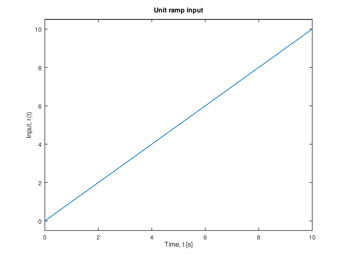 Figure 3.4 Unit ramp
\begin{align*} \mathcal{L}[f(t)] &= \mathcal{L}[t] = \int_{0}^{\infty} t \cdot e^{-st} \, dt\\ \mathcal{L}[f(t)] &= \int V \, du = u \, v - \int u \, dv &&\quad \text{(Integration by parts)} \end{align*} In this case: \[ (v = t), (dv = dt), (du =e^{-st}), \left(u = -\frac{1}{s} e^{-st}\right) \] \[ \int_{0}^{\infty} t \cdot e^{-st} \, dt = -\frac{1}{s} \cdot e^{-st} \cdot t - \int_{0}^{\infty}-\frac{1}{s} e^{-st} \, dt \] \begin{align*} F(s) &= 0 - \left(-\frac{1}{s^2}\right)\\ F(s) &= \frac{1}{s^2} \end{align*}
- Example No.4 Laplace Transformation of a impulse.
Show $ft = \delta(t)$ transforms to $F$ (s) = 1.
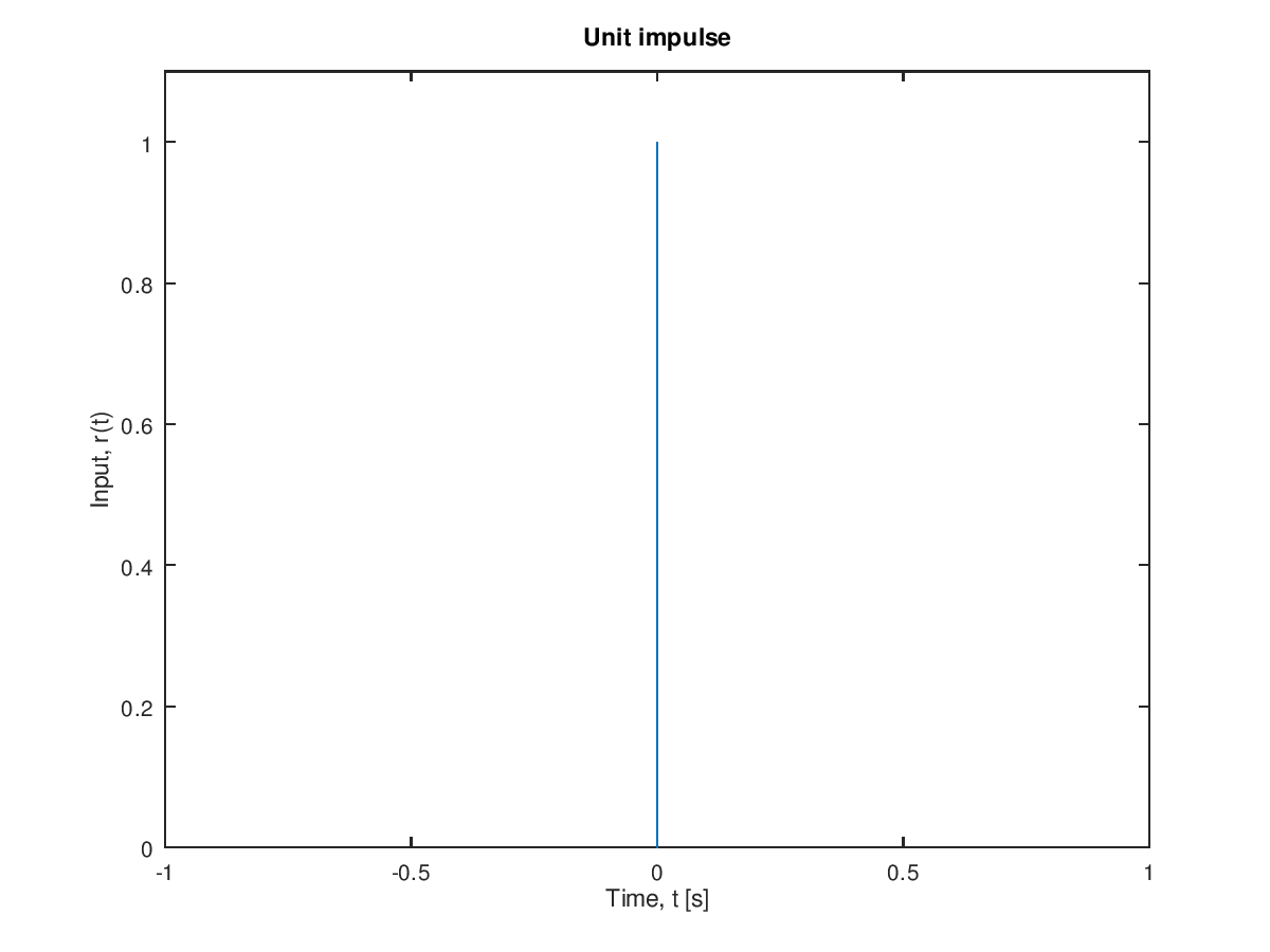 Figure 3.5 Unit impulse
\begin{align*} \mathcal{L} &= [f(t)] = \int_{0}^{\infty}f(t) e^{-st} \, dt \\ F(s) &= \int_{0}^{\infty}\delta(t) e^{-st} dt \end{align*} Since $\delta(t)$ only exists at time $t = 0$ \begin{align*} F(s) &= e^0 = 1 \\ F(s) &= 1 \end{align*}
More examples on in the next tab.
Laplace Transform revision
- Note: We do not need to use the Laplace Transformation function to find the Laplace Transform of Time domain equations. In general we only need to use the Table of Laplace Transforms or software to do the transformations e.g. Matlab, MathCad etc. For completeness here are a few examples of transforming time domain equations $f$ (t) into their Laplace equivalents $F$ (s).
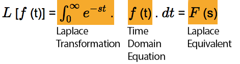
The Laplace Transformation is defined as
$L$ [$f$ (t)] = $\int_{0}^{\infty} e^{-st}$ . $f$ (t) . $dt$ = $F$ (s)
Where $f$ (t) is the time domain equation being transformed.
Any number ( constant ) or mathematical equation can be transformed from the time domain to the Laplace domain using the above formulae.
Usually, lower case letters and the variable $t$, representing time, are used in the time domain equations. Upper case letters and the Laplace operator $s$ are used in the Laplace domain equations. e.g.
\begin{array}{|c|c|} \hline \text{Time Domain} & \text{Laplace Domain} \\\hline f (t) & F (s) \\\hline y (t) & Y (s) \\\hline g (t) & G (s) \\\hline \end{array}- Example No.1
Laplace Transformation of a constant $a$.
\begin{align*} f(t) &= a\\ F(s) = \mathcal{L} [f(t)] &= \int_{0}^{\infty} e^{-st} \cdot a \, dt\\ &= -\frac{a}{s} e^{-st}\\ &= 0 - (-\frac{a}{s})\\ &= \frac{a}{s} \end{align*}
- Example No.2 Laplace Transformation of a unit step ( step size = 1 ).
\begin{align*} f(t) &= 0 &&\qquad t < 0 \\ f(t) &= 1 &&\qquad t > 0 \\ \end{align*} Show the above transforms into the Laplace domain as
\[ F(s) = \frac{1}{s} \]
\begin{align*} \mathcal{L} [f(t)] &= \int_{0}^{\infty} e^{-st} \cdot 1 \, dt \\ \mathcal{L} [f(t)] &= - \frac{1}{s} e^{-st} \left. \right|^\infty_0 \\ F(s) &= 0 - \left(-\frac{1}{s}\right) \\ F(s) &= \frac{1}{s} \end{align*}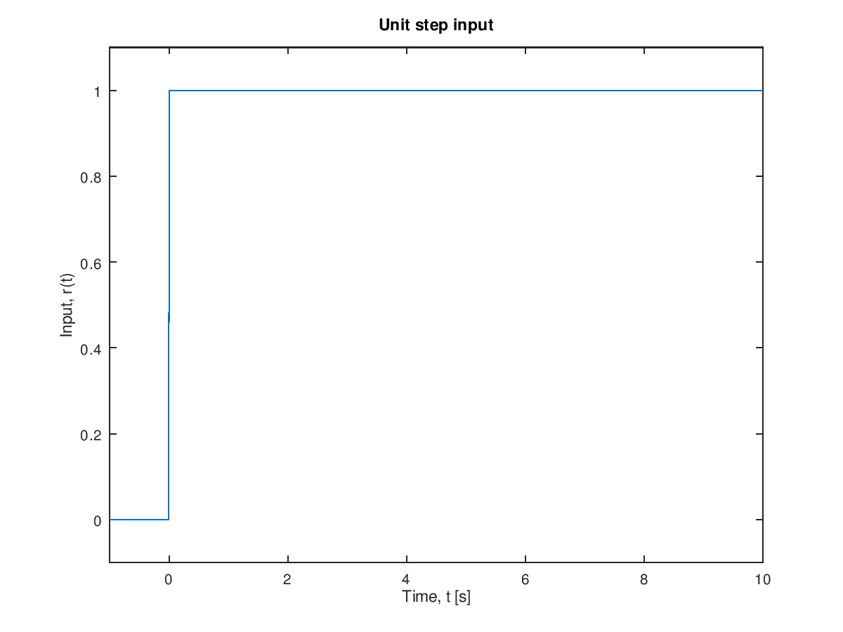 Figure 3.3 Unit step
- Example No.3 Laplace Transformation of a unit ramp ( increase 1 uni per second ).
-
- Example No.9 A closed loop system.
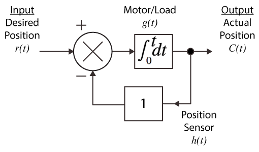 (a) $t$ domain
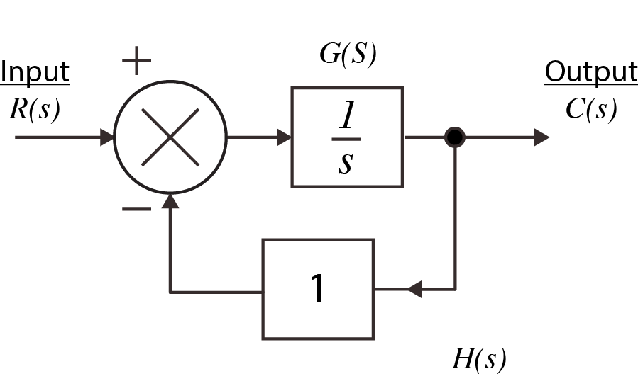 (b) $s$ domainFigure 3.8 Closed loop system
The basic rules for manipulating Laplace Transforms are:
- The basic are:
1. The addition of two time domain functions becomes the addition of the two Laplace transforms. \[f_1(t) + f_2(t) \quad \rightarrow \quad F_1(s) + F_2(s)\] 2. The subtraction of two functions becomes the subtraction of their two Laplace transforms. \[f_1(t) - f_2(t) \quad \rightarrow \quad F_1(s) - F_2(s)\] 3. The multiplication of some function by a constant becomes the multiplication of the function by the same constant. \[a \cdot f(t) \quad \rightarrow \quad a \cdot F(s)\] 4. A function which is delayed by a time $T$ seconds, i.e $f(t)$, becomes $e^{-Ts} \cdot F(s)$ for values of $T$ greater than zero.
5. The first derivative of some function becomes $s$ times the Laplace transform of the function. \[\frac{d}{dt}f(t) \quad \rightarrow \quad s \cdot F(s)\] 6. The second derivative of some function becomes $s^2$ times the Laplace transform of the function. \[\frac{d^2}{dt^2}f(t) \quad \rightarrow \quad s^2 \cdot F(s)\] 7. The $n^\mathrm{th}$ derivative of some function becomes $s^n$ times the Laplace transform of the function. \[\frac{d^n}{dt^n}f(t) \quad \rightarrow \quad s^n \cdot F(s)\] 8. The first integral of some function becomes 1/s times the Laplace transform of the function. \[\int_{0}^{t} f(t) \, dt \quad \rightarrow \quad \frac{1}{s} \cdot F(s)\]
Note: An equation in the time domain is represented by $f$(t), i.e an equation which varies with time. Lower case letters are used in time domain. An equation in the Laplace or $s$-domain is represented by $F$(s). Capital letters are commonly used for the equations in the $s$-domain.
(Examples Cont.)- Example No.5 Laplace Transformation of an exponential.
Show $f(t) = e^{-at}$ transforms to \[F(s) = \frac{1}{s + a}\] \begin{align*} \mathcal{L}[ f(t) ] &= \int_{0}^{\infty} \cdot e^{- s t} \cdot e^{- a t} \, dt\\ \mathcal{L}[ f(t) ] &= \int_{0}^{\infty} \cdot e^{- ( s + a ) t} \, dt\\ \mathcal{L}[ f(t) ] &= -\frac{1}{s + a} \cdot e^{- ( s + a ) t}\\ F(s) &= 0 - \left(-\frac{1}{s + a}\right)\\ F(s) &= \frac{1}{s + a} \end{align*}- Example No.6 Laplace Transformation of a constant multiplying an equation.
Show $a \cdot f(t)$ transforms to $\; a \cdot F$(s) \begin{align*} \mathcal{L}[ a \cdot f(t) ] &= \int_{0}^{\infty} a \cdot f(t) \cdot e^{-st} \, dt\\ \mathcal{L}[ a \cdot f(t) ] &= a\cdot \int_{0}^{\infty} f(t) \cdot e^{-st} \, dt\\ \mathcal{L}[ a \cdot f(t) ] &= a \cdot F(s)\\ \implies a \cdot f(t) &\rightarrow a \cdot F(s) \end{align*}- Example No.7 A temperature sensor that outputs 1 volt in response to a 1 degree change in temperature. This can be represented in block diagram format in the time ($t$) domain or as a block diagram using a transfer function in the $s$ domain.
Output voltage = input temperature $\times$ sensor gain \begin{align*} v(t) &= r(t) \cdot g(t) \\ v(t) &= r(t) \cdot 1 &&\qquad \text{(time domain equation)} \\ V(s) &= R(s) \cdot 1 &&\qquad \text{(Laplace domain equation)} \end{align*}
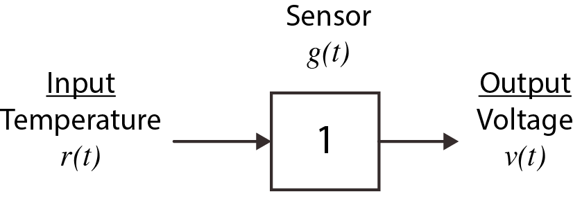 (a) $t$ domain
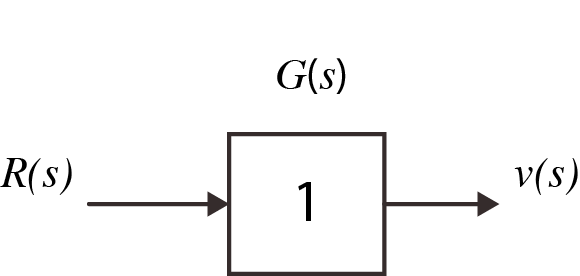 (b) $s$ domainFigure 3.6 Temperature sensor block diagrams - (a) and (b) above
i.e. the equation $g(t) = 1$ transforms to $G(s) = 1$ not $G(s) = 1/s$
Constants in the time domain block diagrams remain as constants when converted to the Laplace domain. This is because the constant is always multiplied by a signal.
- Example No.8 An electric motor which rotates at 10~rad/s for every unit of current.
Because $c(t) = 10 \times i(t)$ transforms to $C(s) = 10 \times I(s)$
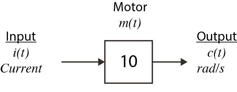 (a) $t$ domain
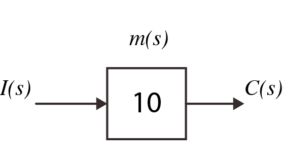 (b) $s$ domainFigure 3.7 Motor block diagram
- Example No.9 A closed loop system.
-
-
Lab Work
Control Engineering 3 - Laboratory Session 2
⬇ Download mlx file
PDF: Control Engineering 3 - Laboratory Session 2
Goals:
Learn how to use MATLAB symbolic toolbox to take Laplace transform of a signal or function given in time-domain.
Learn how to use MATLAB symbolic toolbox to take Inverse Laplace transform of a signal or function given in frequency domain.
Obtaining partial fraction expression for a transfer function using MATLAB
Defining transfer functions for Linear Time-Invariant(LTI) systems in MATLAB
Learning the ways to obtain poles and zeros of a transfer function in MATLAB
Learning to obtain step response for a given transfer function in MATLAB