Hosting Capacity against Overvoltage

Voltage Magnitude Variations in Conventional Distribution Network-1

In a power distribution system, the voltage of a connection point has to be regulated within a certain range at all time (e.g. 0.95 p.u. to 1.05 p.u.).

In a distribution power system, the active and reactive power consumption will result in a voltage drop along feeders, which is lowest with minimum power consumption and highest with maximum consumption.

Voltage Magnitude Variations in Conventional Distribution Network-2

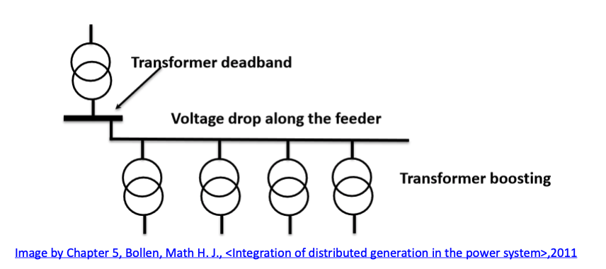
The voltage on secondary side of an HV/MV transformer (e.g., 110/35 kV) is kept within a certain deadband by means of the automatic tap changer(video) of the HV/MV transformer.

Voltage Control in Contentional Distribution Systems

The further away the grid point is from the upstream substation, the lower the voltage on the MV feeder will be.

To compensate for this, MV/LV transformer with different turns ratio are used (off-load tap changer).

The voltage in the distribution network can be boosted by up to 5%

Voltage Operational Band

The operational region of a voltage band may vary: typically a range of 5-10% around the nominal Voltage.

Example: European voltage standard EN50160 specify the votlage variation should be between 90% and 110%

The deadband is normally chosen above the nominal voltage to allow voltage drop along MV and LV feeders.

The Voltage Requirement for All Feeders

Both the highest and the lowest voltages among all feeders should be within the target range.

For a conventional distribution power network with unidirectional power flow

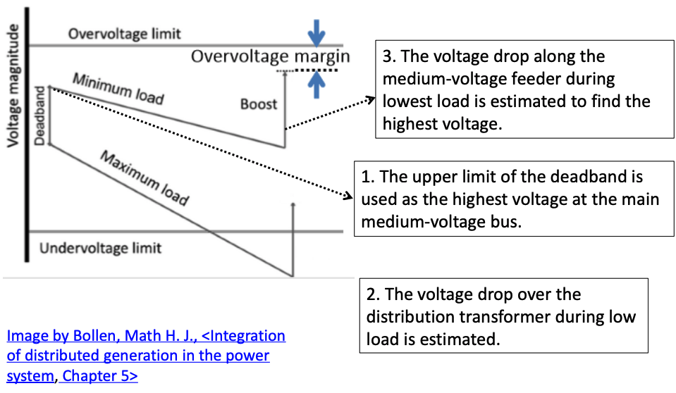
– For any time instant, the highest voltage will be at the distribution substation side when there is no DG.
– The voltage during maximum load for the most remote customer should be above the undervoltage limit.
– The voltage during low load for the nearest customer to the substation, should not exceed the overvoltage limit

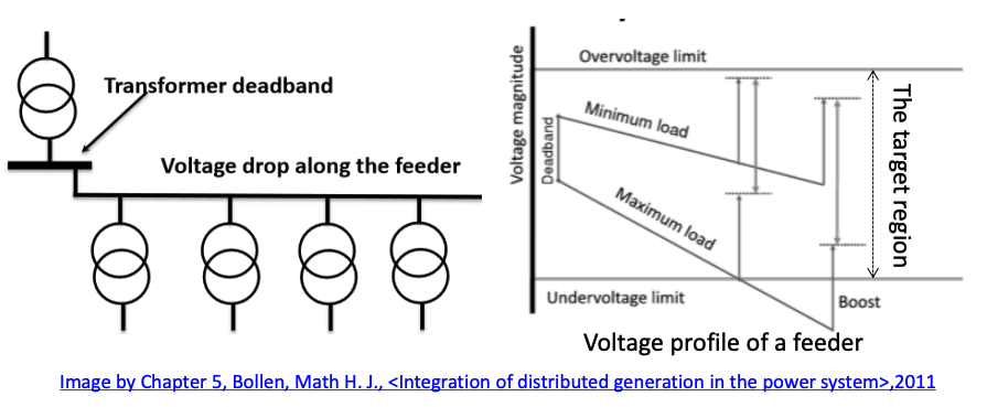
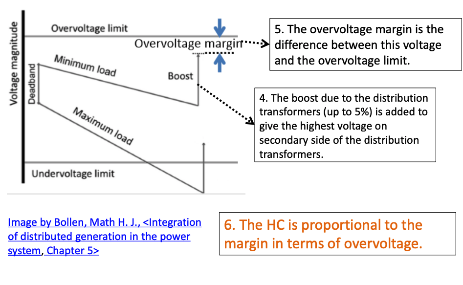
Overvoltage Margin

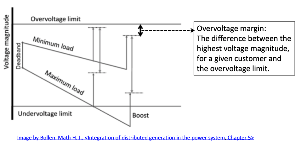
To install a DG, it must be ensured that the overvoltage is not reached at all time.

Obviously, a sufficient overvoltage margin, which is defined above, is needed to allow new DG installment.

Voltage Rise Due to Distributed Generation

The active power injection by the DG to the distribution network will result in a voltage rise.

The relative voltage rise (with unit power factor) can be approximated by

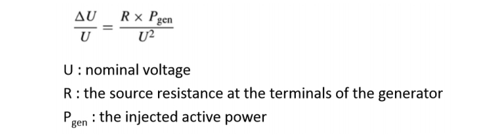
From the above equation, we can tell that

the voltage rise brought by the active power generation is proportional to the injected active power Pgen

the voltage rise brought by the active power generation is proportional to the source resistance R. If the substation voltage is considered to be of an infinite bus, the resistance is proportional to the length of feeder line, which means the terminal voltage of a remote DG could be the highest.

A lower voltage level is likely to have a higher voltage rise (in per unit) as thepower lines are more resistive.

Host Capacity Against Overvoltage

Hosting Capacity (HC): The maximum amount of generation that can be connected without unacceptable quality or reliability for other customers.

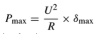
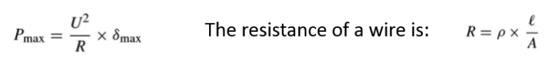
In this case: the HC against the voltage variation should be amount of generation that gives a voltage rise equal to the overvoltage limit.

By manipulating the voltage equation we have below, there is

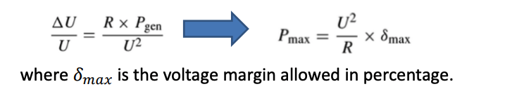
From the above equation, it can be seen that the HC is proportional to the square of the voltage level 𝑈 2 and the voltage margin 𝛿𝑚𝑎𝑥 .

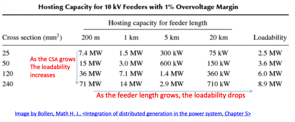
Host Capacity in 10 kV System

From the equations above, the feeder resistance can significantly affect the hosting capacity and the major factors that may impact the feeder resistances are the length and Cross-Sectional Area (CSA). The feeder resistance can be described by

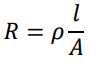
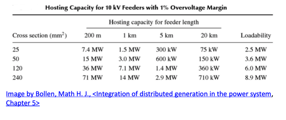
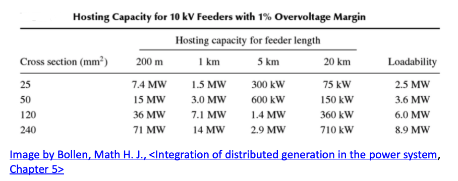
where 𝑙 is the length and A is the CSA. A HC of a 10kV system is illustrated below

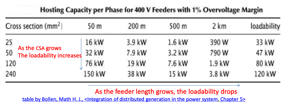
Host Capacity in 0.4 kV System

Using the same principle above, the HC of a 0.4kV system is illustrated below:

Please read Bollen, Math H. J., Integration of distributed generation in the power system, Chapter 5.2

Host Capacity Considering Voltage Limit and Overload

The hosting capacity depends strongly on the feeder size and length.

– For short feeders, large generation can be connected with a voltage rise of less than 1%. The thermal capacity will probably be the main concern.
– For cables longer than several kilometers, the voltage rise is more likely to be the limiting factor, especially for long, small cross-sectional cables.

In short:

For short cables, the maximum load will be likely to limit the host capacity.

For long cables, the voltage rise will likely set the hosting capacity.

Estimating the Hosting Capacity against Overvoltage -Steps breakdown - 1

The step breakdown of how to calculate the HC against over voltage is shown as follows:

Estimating the Hosting Capacity against Overvoltage -Steps breakdown - 2

Example: estimate the HC against overvoltage - 1

For a village where a PV array is to be installed, the network condition that is known before the instalment of the prospected DG is as follows:

The location is connected to the distribution substation via 5 km feeder at 10 kV

The distribution transformer deadband is between 102% and 104%

The distribution transformer voltage drop at low load is 3%.

The boosting due to the distribution transformer is up to 5%

Question: what is the HC against overvoltage according to the table below?

Example: estimate the HC against overvoltage -2

This gives a maximum voltage in LV network equal to 104%-3%+5%=106%

The overvoltage limit is 110%.

The resulting overvoltage margin: 110 – 106 = 4%

The hosting capacity is four times the amount given in the Table below.

Since the connecting feeder is 5 km at 10 kV, the HC for 1% overvoltage margin is 300kW

Therefore, the HC against overvoltage is 300 kW × (4% ÷ 1%) = 1.2 𝑀W

Increasing Hosting Capacity against Overvoltage

Increasing the Host Capacity (against overvoltage) - 1

New or stronger feeders:

– Adding more copper in the form of more or stronger lines, will in almost all cases result in a higher hosting capacity.
– Dedicated feeder in case of larger units connected to weak parts of the grid are a commonly used solution.

Alternative methods for voltage control:

– A load-dependent boosting method would be able to increase the voltage during high load, while not impacting the voltage during low load.
– Automatic tap changers: the tap changer can automatically step down the taps when the voltage is high, but the available steps are limited.
– Power electronics technology: the use of continuous control on the transformer voltage can further narrow the deadband.

e.g. - The use of a Solid-state transformer can provide constant voltage supply independent of the load change.

Increasing the Hosting capacity -2

Accurate measurement of the voltage magnitude variations

- By obtaining more accurate information on the actual voltages over a period of time, the network operator is able to allow more DG to be connected without taking conservative decisions to reject more DG integration.

Allowing higher overvoltage

– With DG, higher overvoltage and lower undervoltage limits could be used to increase the hosting capacity.
– This approach is perhaps the most straight forward, the impact of higher overvoltage limit is a direct increase in the overvoltage margin.
– The drawback is also obvious, it may result in a reduction of power equipment lifespan or mal-fuctioning.

Increasing the Hosting capacity -3

Overvoltage Protection

– Tripping DG when the terminal voltage comes too close to the overvoltage limit is also an easy option.
– The drawback is that the disconnection of an entire DG unit usually means cutting off more DG power generation than necessary. Extra loss of free energy will be incurred to the DG owner.

Overvoltage Curtailment

This is an upgrade version of overvoltage protection scheme.
– A continuous curtailment scheme in which the production is reduced when the voltage gets closer to the limit so there is no need to cut off a DG completely.
– It makes up the drawback of the overvoltage protection scheme.
– Such real-time control over DGs require reliable and timely communication between the controller and DG. Unexpected communication delay and improper design may lead to oscillations of system voltage.

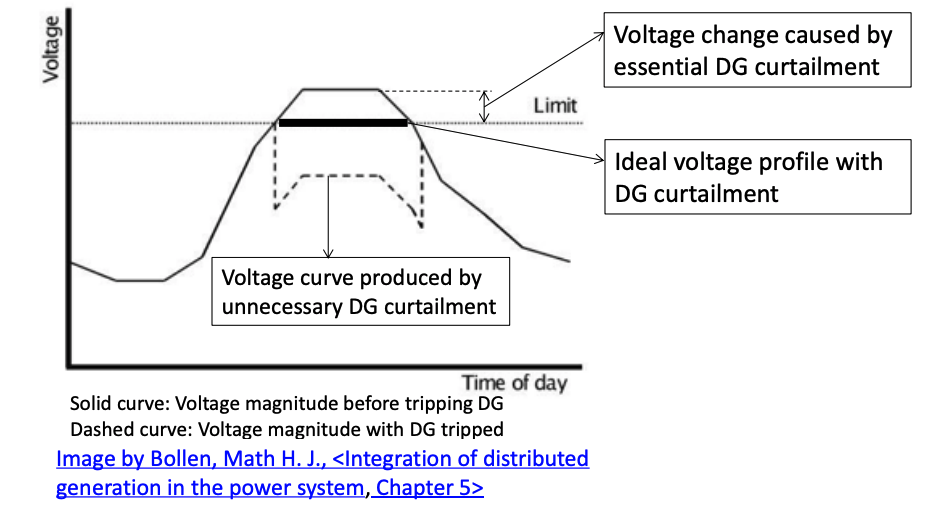
The difference between overvoltage protection and overvoltage curtailment

The drop of DG power can certainly reduce the voltage when there is an overvoltage; but the cost is “dumping” the clean and free energy. The most ideal scenario is to reduce DG output and let the voltage stay at its upper limit, which is demonstrated below:

Increasing the Hosting capacity -4

Distributed Generation with voltage control

– DG operate in a mode to control the amount of reactive power consumed or injected into the grid.
– Use reactive power control to mitigate the voltage variation.
– The control of reactive power might not be very effective when the voltage level is low.
– Extra rating is required for the DG
– Improper control may result in an voltage oscillation itself

Increasing the minimum load

– Charging electric cars in low load conditions is a promising way to accommodate excessive DG power.
– Dedicated battery storage, use a market-bases scheme where different loads and generators put in bids for consumption and production.
– Electric vehicles or battery storage system are still expensive
– Infrastructure investment is in need

DG and Fault Current

Introduction to Fault in Power System

Any failure in a power system which causes short circuit of a section is called a fault.

This short circuit creates a low-impedance path through which fault currents greater than normal condition can flow.

As these fault current magnitudes can be many times larger than normal, they may cause damage to the power system equipment.

What else a fault can cause to a power system?
 - an outage.

Damages Caused by a Fault

These damages could be categorized into electrical and mechanical damages.

From the electrical view point, excessive current flow may cause thermal damage to solid insulation or metallurgical damage to conductors.

Mechanical damage could be produced from high magnetic forces due to the flow of fault current in parallel windings or bus bars.

Why to analyse a fault in a distribution power network?

The magnitude of fault current should be calculated for

– appropriately selecting the equipment rating
– adjusting the settings of protection devices
– sizing the circuit breaker interrupting current capability.

Damages Caused by a Fault

Faults in a power system can be a result of many reasons. They can be both improper human inventions and a consequence of unexpected natural incidents, which includes (but not limited to):

Overvoltage caused by lightning or switching may produce flashover through the air or failure of internal solid or liquid insulation in equipment.

Trees falling over the transmission lines

Accidental contact of birds or other animals between two phases or one phase and a grounded object may cause temporary or permanent faults.

Reduced air gap clearances between the phases or a phase and tower or other grounded object may result in a temporary short circuit. This can be caused by wind, icing, etc.

In a distribution power network, all the above may happen

Types of Faults in a 3-Phase System

In terms of the number of phases involved in the short circuit, the faults are categorized as

– Symmetrical: three-phase short circuit
    • With contact to the ground
    • without contact to the ground
– Unsymmetrical:
    • phase-to-phase
    • phase-to-ground

Introduction to Symmetrical Faults in Power Systems

A symmetrical fault involves a three-phase short circuit, with or without contact to the ground.

– A technical 3-phase fault rarely happens in power systems as it is practically unlikely to have 3 phase power lines short at exactly the same time and the same position.
– A three-phase symmetrical fault causes highest fault current magnitude when a bolt fault (fault with 0 resistance) happens.
– Whether a power system can survive after a 3-phase bolt fault, as the worst case of an electrical fault, is one of the major concern in terms of system design for many mechanical and electrical aspects.

Introduction to Unsymmetrical Faults in Power Systems

An Unsymmetrical(asymmetrical) fault affects one or two phases of a three-phase system

– More than 95% of all faults
– Lower fault current intensities compared to symmetrical faults
– Concerns system stability considerations, relay setting and singlephase operations (switching, for instance)

Fault Calculation

To simplify the calculation of fault current, some assumptions are conventionally made:

The loads do not actively contribute to fault current (this assumption does not apply to rotating machines).

The voltages at all points of the network are assumed to be at nominal level (1 p.u.) where the fault occurs.

No current flows in the network prior to fault.

The transmission line series resistances and shunt admittances are neglected.

Symmetrical 3-phase fault with zero fault impedance is considered in the analysis, which is most severe and pessimistic case from engineering point of view.

Fault Analysis - Symmetrical (three-phase) fault

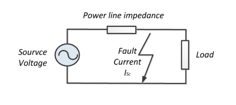
Using Thevinin Equivalent, the 3-phase fault modeling can be simplified as illustrated below:

The fault current is supposed to be produced by the source voltage. In a conventional power network, this voltage is produced the power grid, which is the aggregation of all the generators in connection.

The impedance of network between the source and the fault determines the fault current and the rating of the Circuit Breaker (CB) that should be used.

Fault level

At any given point of the network “the fault level” is the maximum current that would flow in the case of a short circuit (fault). It can be either measure

– In real unit (MVA), or
– In per unit

Assuming that the voltage was equal to its nominal value prior to the fault:

The fault level is defined as

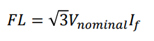
,where 𝐼𝑓 is fault current and 𝑉𝑛𝑜𝑚𝑖𝑛𝑎𝑙 is the nominal voltage of the fault location. In a per unit system, there is

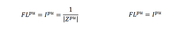
,where Z is the fault impedance between the fault location and the source of the fault current.

Example – Fault Calculation - 1

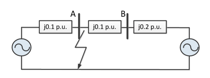
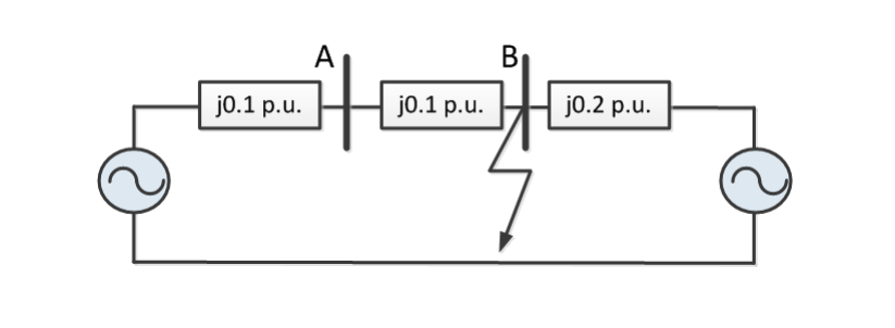
The diagram below shows an embedded synchronous generator connected to a large power system through a distribution network. The fault level at the near end of this network is 500 MVA at zero power factor (i.e. X/R = inf). The impedances of the grid side, between A and B, DG are is j0.1 p.u., j0.1 p.u. and j0.2 p.u., respectively.

If the network is operating at nominal voltage and the load current is negligible, what is magnitude of the current that would flow if faults were to occur at the end of the feeders?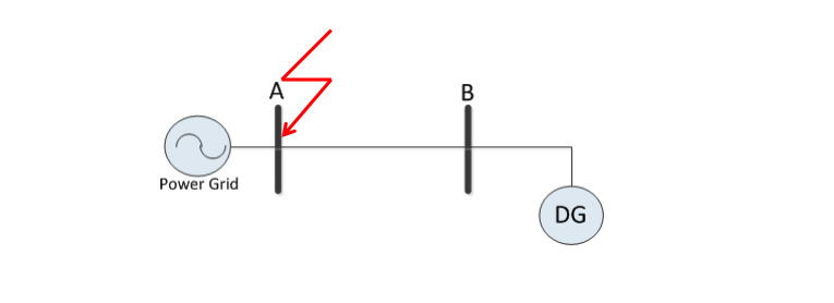

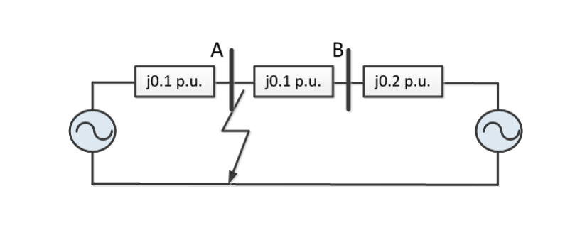
Example – Fault Calculation -2

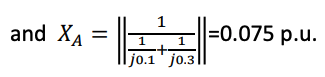
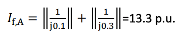
The equivalent circuit for fault calculation is shown above. The large power system has been replaced by its Thevinin equivalent with the impedance. Since the network operates at nominal voltage and the load current is assumed negligible, both voltage source has been set at 1.0 p.u.. The magnitude of the fault current at Bus A is given by

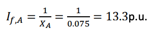
where XA is the parallel combination of the impedances of both sides, which are j0.1 p.u. and j0.3 p.u.

Example – Fault Calculation - 3

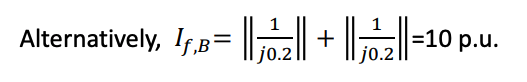
Alternatively, the fault current can be considered as the sum of the fault current from both sides individually and calculated as

Example – Fault Calculation - 4

The magnitude at point B is

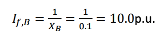
where 𝑋𝐵 is the parallel combination of the impedances of both sides, which are j0.1 p.u. and j0.3 p.u

Faulty Behavior in a Distribution Network

In a meshed power distribution network, the fault current can come from all the live sources. A DG, if alive, could be a potential source as well. The following example shows the fault level and C before and after DG is connected to Bus E.

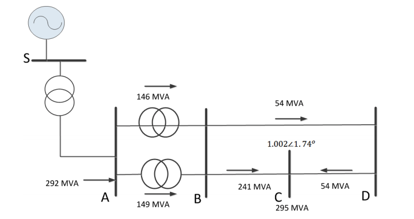
Before the DG connection, Fault level in MVA for a 3-phase fault at Bus C is contributed by all buses in this system. The arrow shows the direction of the fault currents. (assume there is no load before the fault)

Faults: Application to a Distributed Generation Scheme

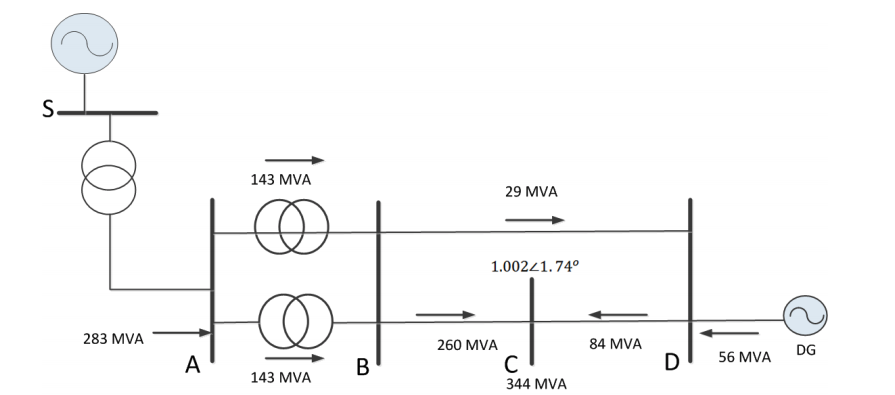
Fault level in MVA for a balanced 3-phase fault at Bus C is contributed by allbuses in this system, including the DG. The arrow shows the direction of the fault currents. (assume there is no load before the fault).

Comparing the previous case without the DG, the total fault current has been significantly increased due to contribution of the DG.

DG and Stability

Introduction to Power System Stability

Stability is probably one of the most profound issue for power system studies. For some aspects, there are still unknown issue without a solid conclusion in theory.

There are many definition of stability.

One of the definition for power system is the ability of a system to return back to a steady-state condition after a disturbance.

Stability for a synchronous machine in a power network refers to recovering its synchronous speed after a disturbance due to changes in the input or output power.

Since disturbance, more or less, is supposed to be coming into power system all the time, stability may be simply considered as if a power system is capable of staying at a close adjacency of certain operational region at steady state.

For the integration of renewable power generation to a power grid, the issue may involve may specific dimensions. One of them concern refers to maintaining the synchronism between the various parts of a power system.

Stability - 1

Stability is one of the major concerns in power system planning and operation.

A stable power system must provide reliable power within the acceptable voltage and frequency range for its consumers.

Instability (loss of synchronism) in part of an interconnected power system may lead to the propagation of the problem by cascading effect and may cause power outages or even complete blackout of the network.

The power balancing for a synchronous generator

In synchronous generator units (in steady-state and ignoring the losses):

The mechanical power provided by the prime mover = electrical power produced by the generator

In mechanical term: The accelerating torque (applied to the shaft by the prime mover) = The decelerating torque (caused by the production of electric power)

At equilibrium for a synchronous generator:

The net torque is 0

The shaft rotates at a constant speed.

The angle between the rotor field and stator field is constant.

Modeling Power Transfer between Two Buses

One of the concern about DG stability is that if a fault happens, will the DG still be able keep stability after the fault cleared, which is illustrated below.

The simplified stability analysis can be considered with a single-infinite bus scenario as illustrated where is the power grid is modeled as an infinite bus in connection with an impedance XL. The grid angle can be defined as 0 for simplicity.

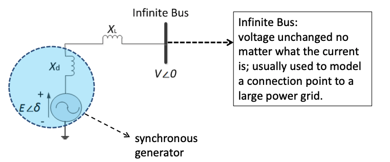
A Synchronous Generator (SG) based DG is connected to an infinite bus through a transformer and a transmission line with a total reactance of XL .

So the total reactance between the bus and the SG emf is

X = Xd + XL

Modeling Power Transfer between Two Buses

The voltage at the infinite bus (V) is constant and considered to be the voltage reference.

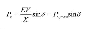
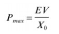
the real (active) power transmitted to the infinite bus (Pe) is

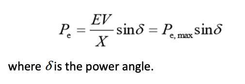
Since once a system is established, the change of emf E, grid voltage and the total reactance is very limited, the power exchange between the generator and grid is therefore determined by δ, the angular difference between the emf and grid voltage ; hence the terminology of “power angle”.

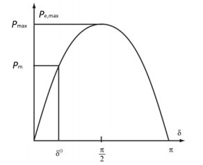
The Power Angle Curve - Power Vs. Power Angle

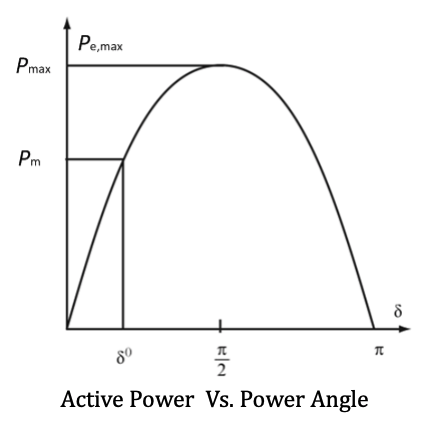
Based on the power angle equation above, the curve of active power P versus the power angle δ (P- δ curve)should be a sinusoidal waveform as shown, where Pe,max is the peak value of the electrical power is defined as Pe,max; the energy source power input is PM and the operational power angle is 𝛿0.

For a synchronous generator connected to an infinite bus, the power angle δ has to be below 90 degree to maintain stability at steady state.

Stability Analysis in a 2-bus System - 1

Considering a Synchronous Generator (SG) based DG is connected to the grid with two parallel power lines as below, a equivalent circuit is created.

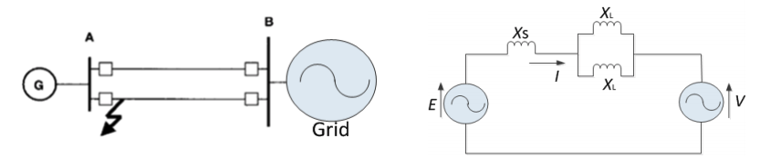
Before the fault, the total impedance between the SG emf and the infinite bus is

Xs is the source impedance (stator impedance for synchronous generator), again the power angle curve can be shown as below.

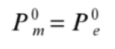
For steady state the input source power Pm0 at steady state should equal to the electrical power Pm0 before any fault happens, if the system is assumed as lossless for simplicity:

Stability Analysis in a 2-bus System - 2

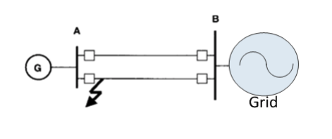
During a fault:

For a single-infinite double line system shown above, when a 3-phase bolt fault (0 impedance fault) occurs at Bus A :

The voltage at bus A become 0.
• The generator cannot inject power into the grid (0 voltage cannot deliver any power)
• The mechanical torque unchanged so the net torque becomes a none-zero value. The power balance is lost.
• Rotor starts to accelerate
• Rotor angle δ starts to increase.

Stability Analysis in a 2-bus System - 3

To clear the fault, the circuit breaker across the fault line has to be open as shown below.

Therefore, the equivalent reactance between the emf of the generator and the grid is changed as shown in the equivalent circuit.

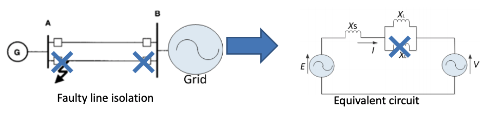
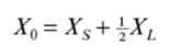
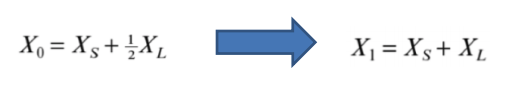
After the fault clearance, with a parallel power line tripped, the post-fault total impedance X1 becomes greater than pre-fault X0.

Since the total impedance has been changed, the P-δ curve will be consequently changed as well.

Stability Analysis in a 2-bus System - 3

Considering the new impedance after the fault is

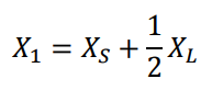
, which is less than what was in the pre-fault condition, therefore

As is shown above, the post-fault P-δ curve will be lower than the pre-fault curve as the reactance value on the denominator of the power expression has increased due to the disconnection of one power line.

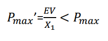
As the DG capacity may grow large or the power lines grows longer, the postfault P’ max can become less than the input mechanical power as

Pmax' < Pmo

, which means the strength of the connecting grid is very weak that the mechanical torque can never be balanced by the electrical. The generator will loose synchronism and the system will be unstable after a severe fault.

Please try Tut 3-9

Stability Analysis in a 2-bus System - 4

The new electrical power transferred to this grid is larger than the mechanical power input .

Decelerating torque is larger than accelerating torque.

The rotor slows down.

The rotor angle continues to increase for a while because of the kinetic energy stored during the fault.

The input power and the electrical power output will eventually reach a new Equilibrium point.