Wk 5
-

2D Strain Analysis
In this lecture, you will learn about the relationship between principal stresses (studied earlier) and principal strains. You will learn about the different strain gauges used to measure strains and how to compile a Mohr circle of strain from measured strain values. The principal strains and the maximum shear strain can be scaled from the Mohr circle of strain. These values, along with known material properties, can be substituted into simple equations to obtain the principal stresses. -
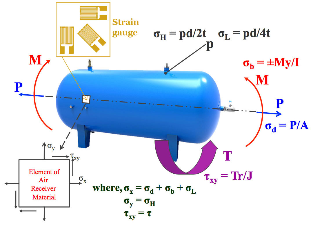
A 2D Stress Analysis application
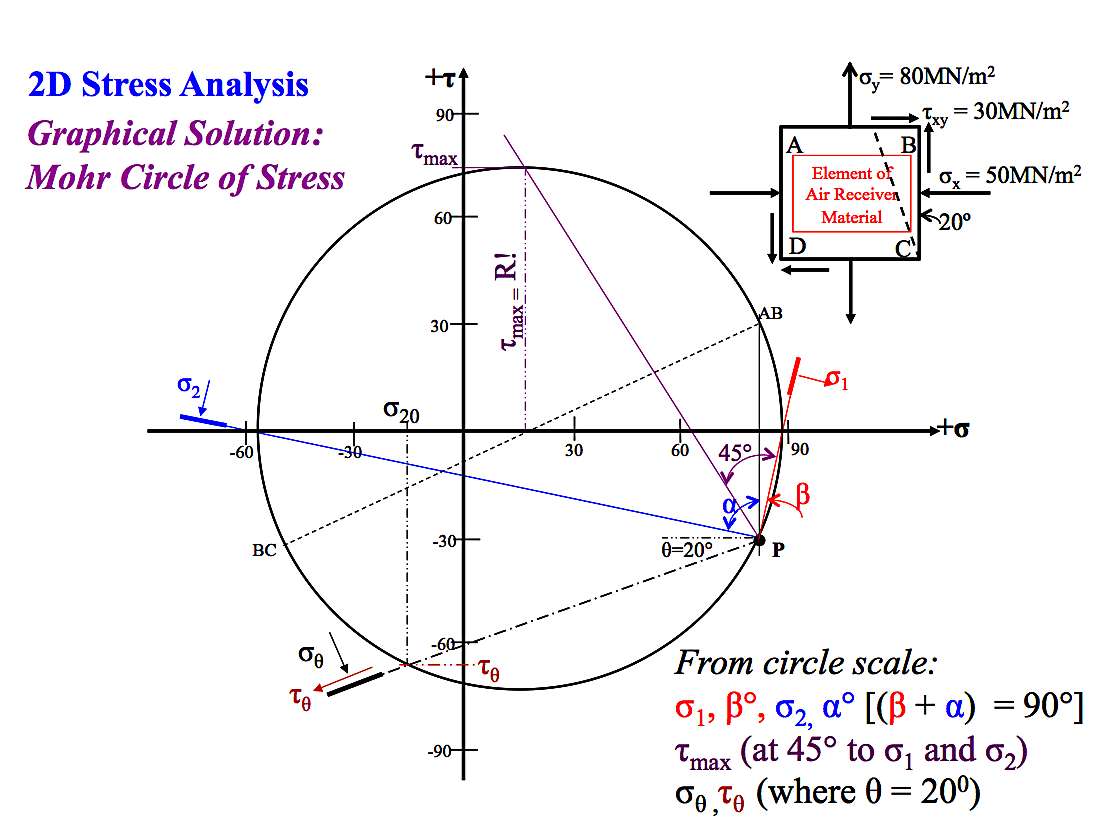
Analytical Solution
- $$ \large \sigma_\theta = \frac{\sigma _x - \sigma _y}{2} + \frac{\sigma _x - \sigma _y}{2} cos \; 2 \theta + \tau \; sin \; 2 \theta \quad \small \textbf{Eqn(1)} $$
$$ \large \tau_\theta = \frac{\sigma _x - \sigma _y}{2} \; sin \; 2 \theta - \tau \; cos \; 2 \theta \quad \small \textbf{Eqn(2)} $$
$$ \large \text{tan} \; 2 \theta = \frac{2 \tau}{\sigma _x - \sigma _y} \quad \small \textbf{Eqn(3)} $$
$$ \large \sigma_1 = \frac{\sigma _x + \sigma _y}{2} + \sqrt{\Bigg( \frac{\sigma _x - \sigma _y}{2} \Bigg)^2} + \tau^2 \quad \small \textbf{Eqn(4)} $$
$$ \large \sigma_2 = \frac{\sigma _x + \sigma _y}{2} - \sqrt{\Bigg( \frac{\sigma _x - \sigma _y}{2} \Bigg)^2} + \tau^2 \quad \small \textbf{Eqn(5)} $$
$$ \large \tau _{max} = \frac{\sigma _1 - \sigma _2}{2} \quad \small \textbf{Eqn(7)} $$
- $$ \large \sigma_\theta = \frac{\sigma _x - \sigma _y}{2} + \frac{\sigma _x - \sigma _y}{2} cos \; 2 \theta + \tau \; sin \; 2 \theta \quad \small \textbf{Eqn(1)} $$
-
2D Stress Analysis here
- Normal strain or direct strain is the change in length (dimension)/original length (dimension) and is denoted by $ \varepsilon $ (+ tensile, - compression).
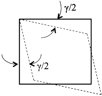
Shear strain is a measure of the change of shape - taken as the total angular change in any right angle, denoted $ \gamma $. Taken as positive corresponding to +ve shear stress, and vice versa.- Material Properties – Elastic Behaviour:
The strains at a point in a 2D stress system can be analysed in a similar manner to that for stresses (but more complex), and the following expressions apply:
 Also $ \huge \frac{\tau _{xy}}{\gamma _{xy}} $ = constant = G (Modulus of Rigidity, N/m2)
Also, recall Hooke’s law: $ E = \huge \frac{\sigma}{\varepsilon} $ ($ E $ = Young’s Modulus of Elasticity, N/m2)
And, $ E $ = 2G(1 + ν) (ν = Poisson’s ratio = $ \large \varepsilon _{Lat} / \varepsilon_L $ )
$ \large \quad \varepsilon _\theta = \frac{\LARGE \varepsilon _x + \varepsilon _y}{2} + \frac{\LARGE \varepsilon _x + \varepsilon _y}{2} \; cos \; 2 \theta \; - \; \frac{\LARGE \gamma _{xy}}{2} \; sin \; 2 \theta $
Similar to stress Eqn(1):
$ \large \sigma _\theta = \frac{\LARGE \sigma _x + \sigma _y}{2} + \frac{ \LARGE \sigma _x - \sigma _y}{2} \; cos \; 2 \theta \; + \; \tau \; sin \; 2 \theta $
$ \quad \bigg( \frac{\LARGE \gamma}{\large 2} \bigg) \large _\theta = \frac{\LARGE \varepsilon _x + \varepsilon _y}{\large 2} \; sin \; 2 \theta - \; \frac{\LARGE \gamma _{xy}}{\large 2} \; cos \; 2 \theta $
Similar to stress Eqn(2):
$ \large \tau _\theta = \frac{\LARGE \sigma _x - \sigma _y}{\large 2} \; sin \; 2 \theta \; - \; \tau \; cos \; 2 \theta $
Plotting values of $ \large \varepsilon _\theta $ and $ \Bigg( \frac{\LARGE \gamma}{\large 2} \Bigg) \large _\theta $ for varying values of $ \theta $ gives the Mohr.Circle of Strain, similar to the Mohr Circle of Stress. - Normal strain or direct strain is the change in length (dimension)/original length (dimension) and is denoted by $ \varepsilon $ (+ tensile, - compression).
-
2D Stress Analysis (cont.)
- The radius of the circle
$ \quad \; = \sqrt{ \Bigg( \frac{\LARGE \varepsilon _x - \varepsilon _y}{2} \Bigg)^2 + \Bigg( \frac{\LARGE\gamma _{xy}}{2} \Bigg)^2 } $Similar to stress Eqn(6):
$ \Large \sqrt{ \Bigg( \frac{\sigma _x - \sigma _y}{2} \Bigg)^2 + \tau ^2 } $
The centre of the circle lies at a distance from the origin $ \frac{}{} $ similar to the stress circle, and the principal strains $ \varepsilon _1 $ and $ \varepsilon _2 $ are:
$ \quad \varepsilon _{1,2} = \frac{\LARGE \varepsilon _x + \varepsilon _y}{\large 2} \pm \sqrt{ \Bigg( \frac{\LARGE \varepsilon _x - \varepsilon _y}{2} \Bigg)^2 + \Bigg( \frac{\LARGE\gamma _{xy}}{2} \Bigg)^2 } $Similar to stress Eqn(4,5):
$ \Large \sigma _{1,2} = \frac{\sigma _x + \sigma _y}{2} \pm \sqrt{ \Bigg( \frac{\sigma _x - \sigma _y}{2} \Bigg)^2 + \tau^2 } $
$ \quad \normalsize \text{tan} \; 2 \beta = \frac{\Large\gamma/2}{\Large (\varepsilon _x - \; \varepsilon _y) \; / \; 2} $Similar to stress Eqn(3):
$ \large \text{tan} \; 2 \theta = \frac{2 \tau}{\Large\sigma_x - \sigma_y} $
The plane of maximum shear strain is at 45° to the principal plane.2D Strain Analysis - Strain Measurement
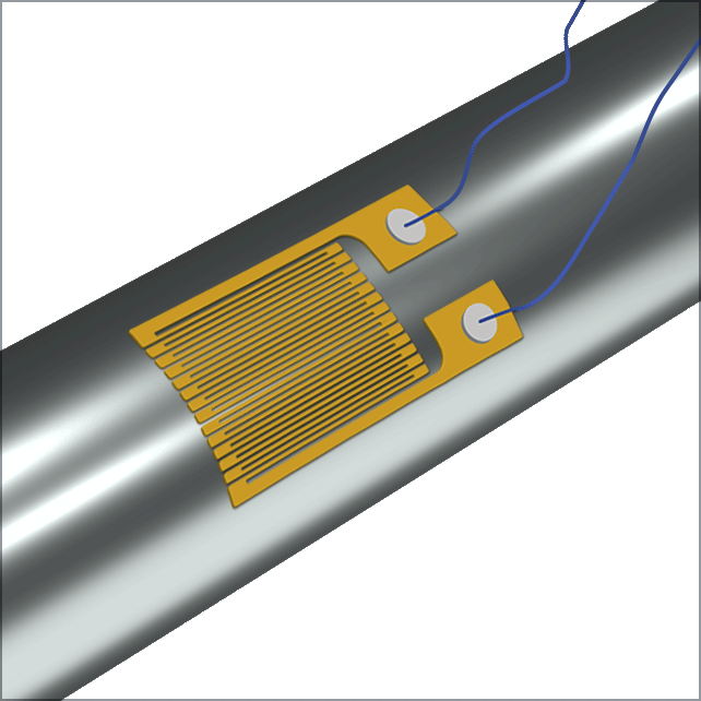
Strains at a point in a loaded component cannot be measured directly, but their effect in the form of direct strains can be measured by means of strain gauges or extensometers and stress calculations can be carried out from these measurements.
The aim of the strain measurement is to find the principal stresses (and generally the major value) and their directions relative to some given reference direction.
If the principal stress directions are known, a pair of strain gauges in these directions at a point will give the principal strains from which the principal stresses can be found by the usual stress-strain equations in two-dimensions. - The radius of the circle
-
Mohr’s Circle of Strain – Calculation of Stresses
- The principal strains are ε1 and ε2 as shown, the directions being at angle θ to the reference plane B by use of the pole point as shown.
Having found the principal strains ε1 and ε2, the principal stresses σ1 and σ2 are obtained quite easily as follows:
$ \large \varepsilon _1 = \frac{1}{E} \Bigg[\sigma_1 - v \sigma_2 \Bigg] \quad \small \textbf{Eqn(1)} $
$ \large \varepsilon _2 = \frac{1}{E} \Bigg[\sigma_2 - v \sigma_1 \Bigg] \quad \small \textbf{Eqn(2)} $
From Eqn. (1):
$ \large E \varepsilon _1 = \sigma _1 - v \sigma _2 $
$ \large \therefore \sigma _1 = E \varepsilon _1 + v \sigma _2 \quad \small \textbf{Eqn(3)} $
From Eqn. (2):
$ \large \sigma _2 = E \varepsilon _2 + v \sigma _1 \quad \small \textbf{Eqn(4)} $
From Eqn. (3) and (4):
$ \large \sigma _1 = E \varepsilon _1 + v (E \varepsilon _2 + v \sigma_1) $
$ \large = E \varepsilon _1 + v E \varepsilon _2 + v^2 \sigma_1 $
$ \large \therefore \quad \sigma _1 = \frac{E}{1 - v^2} [ \varepsilon _1 + v \varepsilon _2 ] \; \; \small \textbf{Eqn(5)} $
$ \large \therefore \quad \sigma _2 = \frac{E}{1 - v^2} [ \varepsilon _2 + v \varepsilon _1 ] \; \; \small \textbf{Eqn(6)} $
Where E = Young’s Modulus of Elasticity (N/m2) and ν = Poisson’s ratio for the component material.
Strain Measurement (cont.)
- If however the principal stress directions are unknown, a pair of strain gauges arranged at a known angle to each other at a point, do not give sufficient information to enable a Mohr Circle of Strain to be constructed for the strains at that point.
The normal strains are known from the gauge readings but as the associated shear strains cannot be obtained from the readings, the Mohr Circle cannot be constructed.
Thus when principal stress directions are unknown, three strain gauges arranged at known angles to each other at a point (e.g. a strain rosette) will give the minimum data necessary to construct a Mohr Circle for the strain system at the point.
Assume the typical strain gauge rosette shown gives strain readings εA, εB, and εC. Thus strains εA, εB, and εC, and angles α and β would all be known.
 A typical strain gauge
rosette arrangement.
Mohr’s Circle of Strain – Method of Construction
- Please watch the videos below. When you finish it, carry on with the text below.
- ⬇ Download worked example
-
-
Tutorials
- ⬇ 2D Strain Analysis