3 Algebra

Algebra is all about manipulating formulae, moving terms around, adding or subtracting things from both sides of an equation, and other related techniques.

However, the key feature of algebra is the use of letters to represent unknown values. This makes it more advanced than just standard arithmetic.

3.1 Operations and expressions

This section is designed as a reminder of certain basic techniques; namely using the basic operators (\(+,-,\div,\times\)) and a reminder of powers (also called indices).

3.1.1 Basic Operations of Arithmetic

We might talk of the addition operator \(+\), subtraction operator \(-\), division operator \(\div\) or \(/\), and multiplication operator \(\times\). By operation all that is meant is an agreed procedure (in our cases they will all involve two numbers). We also sometimes need brackets to help clarify unambiguously the order in which the operations should be performed. There is a fifth operator which doesn’t have a symbol, namely exponentiation (just a fancy word for ‘taking powers’). On most calculators this fifth operator is represented by a button that says \(x^y\) or \(x^{\Box}\) or \(\Box^{\Box}\).

An expression is the name we will give to any collection of maths symbols intended to have a value or represent something.

The order in which we perform a calculation is very important, otherwise we may achieve a different answer to someone else.

A point we will keep returning to is the importance of agreed conventions and meanings so that our written maths, equations and solutions are unambiguous.

Take, for example, \[\begin{equation} 9 + 4 \times 3. \tag{3.1} \end{equation}\]

The agreed convention for such an expression is to perform the multiplication (\(\times\)) before the addition (\(+\)). Many of you will have seen an acronym like BODMAS or BIDMAS to help learn this ordering (First to Last).

BODMAS stands for…

Brackets Orders Division Multiplication Addition Subtraction

where Orders refers to powers (i.e. exponentiation)

So for the above expression, (3.1), we need to calculate \(4\times 3 = 12\) and add this to \(9\), resulting in an answer of \(21\).⁴

Beware, however, that it isn’t quite as easy as just learning this one sequence. Luckily you can always just insert brackets to make it obvious.

Unfortunately it’s not always exactly this simple when an expression contains multiple similar or opposite symbols. Division and Multiplication come as a pair and are opposites of each other⁵, as do Addition and Subtraction which are also opposites of each other⁶. If we have an expression made of just \(+\) and \(-\) signs then we should work left-to-right (but still do brackets or powers first as usual). The same applies for \(\times\) and \(\div\) though this is rarer and we often just use brackets.

Here are a few examples of these complicated cases:

• \(3\div 6\times 4\) means \(0.5 \times 4 = 2\)  (left-to-right)
• \(20 \div (5 \times 2)\) means \(20 \div 10 = 2\)  (brackets first)
• \(2-6-(4-3)\) means \(2-6-1 = -5\)  (brackets first)
• \(-4+3-6+8 = 1\)  (left-to-right)

All of these could be made abundantly clear with the addition of extra brackets (sometimes inside each other) but people are often lazy. For example, the first case above could have been written \((3\div 6)\times 4\) to remove any confusion. Or the final one could have been written \(((-4+3)-6)+8\).

Link to Numbas on the web

3.1.2 Expanding brackets

The correct procedure for expanding brackets becomes more complicated the more brackets which are multiplied by each other. At its most simple just one number appears outside a bracket, and you just multiply that one number sequentially by every number inside the bracket, i.e.

\[\begin{equation*} 7\left(3-x+2y\right) = 7 \times 3-7\times x+7\times 2y = 21-7x+14y \end{equation*}\] Notice that if the factor on the outside is negative then we sometimes will get two minus signs, \(--\) which equals \(+\). For example, \[\begin{align*} -4\left(-2+3x-7y\right) & = -4 \times (-2)-4\times 3-4\times (-7y) \\ & = --8-12x--28y \\ & = 8-12x+28y \end{align*}\]

When a bracket is multiplied by a bracket then every combination product of one term from each needs to be calculated and then all combined. So in general, \[\begin{equation*} \left(A+B\right)\left(C+D\right) = A \times C+A\times D + B\times C+B\times D, \end{equation*}\] or for larger brackets \[\begin{equation*} \left(A+B+C\right)\left(D+E\right) = A D+A E+B D+B E+C D+C E. \end{equation*}\] (where all terms on the right are products, \(AD=A\times D\) etc…)

There are a few ways to learn a systematic procedure to ensure no terms are missed, a demonstration video appears below for a specific typical example. However, the main point to remember is that every combination of one term from one bracket with one term from the other bracket must be included in the answer⁷. A method known as the grid method for expanding brackets is particularly worth looking into for anyone who wants to read further.

Alternative direct video link:

https://gcu.planetestream.com/View.aspx?id=3449~4u~vz7dULN7

3.1.3 Powers

Powers are also called Indices, or (occasionally) Exponentiation. Powers are fundamentally just a time-saving notation used to save writing out repeated products.

So we write

• \(a^2\) instead of \(a\times a\),
• \(a^3\) instead of \(a\times a \times a\),
• \(a^8\) instead of \(a\times a \times a \times a \times a \times a \times a \times a\),

This notation is frequently used when performing algebra to re-arrange equations, or to solve for some unknown variable. To help with these manipulations there are a few useful ‘rules’ or ‘laws’ to learn (really they’re just common patterns you can use to simplify quickly).

From this basic definition the three main laws of powers are actually fairly straightforward:

Law 1: For all \(x\) and all \(a,b\), even negative or decimal values… \[\begin{equation} x^a \times x^b = x^{a+b} \tag{3.2} \end{equation}\]

Law 2: For all \(x\) and all \(a,b\), even negative or decimal values… \[\begin{equation} x^a \div x^b = x^{a-b} \tag{3.3} \end{equation}\]

Law 3: For all \(x\) and all \(m,n\), even negative or decimal values… \[\begin{equation} (x^m)^n = x^{m \times n} \tag{3.4} \end{equation}\]

You will have seen these laws before and with repeated use you will no doubt become familiar with them. The intermediate step for anyone not fully familiar with these rules is to at least know that these laws exist, and be able to re-discover them for yourself with a small example.

Here’s a very useful example which uses the powers of \(3\) and \(2\) to work out all three laws!

\[\begin{equation} x^3 \times x^2 = (x \times x \times x) \times (x \times x) = (x \times x \times x \times x \times x) = x^5 \\ \tag{3.5} \end{equation}\]

So, \(x^3 \times x^2 = x^5\) tells us the rule for a product must be to add the powers. Since the only way to get \(5\) from \(2\) and \(3\) is to add them.

The same idea can be used to work out the other laws too:

\[\begin{equation} y^3 \div y^2 = (y \times y \times y) \div (y \times y) = \frac{y \times y \times y}{y \times y} = \frac{y}{1} = y \tag{3.6} \end{equation}\]

We used unknown letter \(y\) here just to illustrate that the name of the unknown isn’t relevant. We see that \(y^3 \div y^2 = y^{3-2} = y^1\) so the rule for division is to subtract the second power from the first. It is perhaps worthy of note that the \(\div\) symbol is just a shorthand for writing out a fraction, so \(y^3 \div y^2\) is just another way of writing \(\frac{y^3}{y^2}\).

Finally, we can again use \(3\) and \(2\) as powers to illustrate the third law.

\[\begin{equation} \left(x^3\right)^2 = \left(x \times x \times x\right) \times \left(x \times x \times x\right) = x^6 \tag{3.7} \end{equation}\]

So we notice that \(\left(x^3\right)^2 = x^{3\times 2}=x^6\) and the rule is that powers raised to powers means we multiply the powers.

There are other patterns, sometimes also called rules or laws, for performing algebra with powers which you will also come across and use at different times. The two main ones are:

• \((xy)^n = x^n y^n\), for example \((2a)^3=8a^3\), and
• \(\left(\frac{x}{y}\right)^n = \frac{x^n}{y^n}\), for example \(\left(\frac{x}{7} \right)^2 = \frac{x^2}{49}\).

Finally these two facts you’ll come across for powers are less rules and more mathematical notation choices:

For all \(x\),

\[x^0 = 1, \]

except when \(x=0\), in which case \(0^0\) is mathematical nonsense.

For all \(x\) and all \(n\),

\[x^{-n} = \frac{1}{x^n}. \]

This can be thought of as a definition of negative powers if you wish.

Example 1

Simplify \[\left(xy^2\right)^3 \div y\]

Answer: First we need to expand the bracket (BODMAS), remembering that every term in the bracket needs to be cubed. So we get \[ (x)^3 (y^2)^3 \div y\] the next step is to use our third power law to rewrite \((y^2)^3\) as \(y^6\). Then finally we use the second power law (about division) to replace \(y^6 \div y\) with \(y^{6-1}=y^5\) giving our final answer of \[ x^3y^5.\] Note that the \(x\) and \(y\) terms are different letters and so are not combinable using the power laws.

Example 2

Simplify \[\frac{3x^2y^3z^{-2}}{(xy^{-3}z)^2} \]

Answer: Again we begin by expanding the bracket on the bottom, we are using the fact that \[ (abc)^2 = a^2b^2c^2 \] to give us \[ \frac{3x^2y^3z^{-2}}{(x)^2(y^{-3})^2(z)^2} \] On the bottom we now need to replace \((y^{-3})^2\) with \(y^{-6}\), using our third law again. So we have reached: \[ \frac{3x^2y^3z^{-2}}{x^2y^{-6}z^2} \] Now we can treat the \(x\), \(y\) and \(z\) parts separately.

Our overall \(x\) terms looks like: \[ x^2 \div x^2 = x^{2-2}=x^0 = 1\] Our overall \(y\) term looks like: \[ y^3 \div y^{-6} = y^{3--6} = y^{3+6} = y^9\] note we were careful here to subtract (not add) \(-6\), so two negative signs gave a \(+\).

Finally our overall \(z\) term will be: \[ z^{-2} \div z^2 = z^{-2-2}=z^{-4}. \] So overall (not forgetting the initial factor of \(3\)) we obtain: \[\frac{3x^2y^3z^{-2}}{(xy^{-3}z)^2}=3y^{9}z^{-4}=\frac{3y^9}{z^4} \] and the \(x\) term disappeared as it was identical on top and bottom (and so cancelled perfectly).

Practice

Simplify these 8 formulae and then put them into 4 matching pairs.

1. \(x \times x \times y \times y \times y^2 \times \frac{1}{z^2}\)
2. \((xyz)^3 x^{-1}z^{-5}\)
3. \(x y^4 z \div y^2\)
4. \(x^3x^{-5}y^2y^{-3}z^{-2}z^1\)
5. \(x^2y^3 \div z^2\)
6. \(\frac{x^{-2}y}{y^2z}\)
7. \(\frac{(xyz)^2}{xz}\)
8. \(\left(xy\right)^2\left(yz^{-1}\right)^2\)

Link to Numbas on the web

3.1.4 Grouping ‘like’ terms

This is one of the key early skills required to perform algebra. We all know that for a sum like \(3-4+8-16+7\), arithmetic can be used to simplify this into a single number (\(-2\) in this example). This is because all the terms are just constants.

If, however, you are presented with the formula \(3-x+8+5x-7\) then the simplification will not be just a number. You need to identify terms which are ‘like’ (or ‘alike’) because they contain unknown variables in exactly the same format as each other. In this example the \(3\), \(8\) and \(-7\) are alike as they are all just constants and don’t mention \(x\). Similarly the \(-x\) and \(5x\) are alike because they are both of the format ‘constant\(\times x\).’ We can combine terms when they will look the same if you overlook different constants on the front. The constant on the front of an unknown variable is called the coefficient, e.g. the coefficient of \(7x\) is \(7\) and the coefficient of \(-4y\) is \(-4\). Terms which have different powers of an unknown variable are regarded as in a different format.

More generally, all of the following are different formats to each other \[\begin{equation*} x, x^2, x^3, x^4, x^{1.5},x^{-7}, xy, xz, xy^2, \ldots \end{equation*}\]

The list of different formats could go on forever, but the key idea is as follows.

Two terms are of the same format if when they are added together you get another object of exactly the same format. When dealing with variables and their powers, they are the same format if they have identical variables and powers.

So \(x^2\) and \(y^2\) are not alike, but \(3xz^2\) and \(-9xz^2\) are alike.

It’s almost always a good idea, before diving into performing algebra and re-arranging an equation, to first group like terms together and combine their coefficients.

Some quick practice

• \(5+x-8+x = -3 + 2x\)
• \(x^2-4x+3+7x=x^2+3x+3\)
• \(8-x^2+2\left(x^2+5\right) = x^2+18\)
• \(x(x-y)+y(z+x)=x^2+yz\)
• \(7x^2-4xy^2+x^2y+3xy-8y^2+xz-xyz+3y^2x = \\ 7x^2-xy^2+x^2y+3xy-8y^2+xz-xyz\)

In all these examples the second version is fully simplified, all presented terms are of different formats. You should check them carefully to see that you agree.

When progressing to more advanced algebra, with formulae that include functions like \(\sin(x)\), and \(\log(y)\) we will need to expand our definition of like terms. The good news is that once functions are involved, only different constants on the front of the function mean terms are alike, otherwise they are different. So \(3\sin(4x) + 7\sin(4x)\) can be combined into \(10\sin(4x)\) but \(3\sin(x)+4\sin(2x)\) cannot be combined.

3.2 Common algebra mistakes

It’s always slightly dangerous to show incorrect algebra, as it might make some poor quality memories for you. However, some errors are so common when working with brackets, powers and fractions that it can still be worthwhile to show you them in action. Make sure to spend longer looking at the ‘Correct algebra’ side of this table. Perhaps even start with the right-hand-side and then look at the left to see how not to do it.

Common mistake (i.e wrong!)	Correct algebra
\(\left(2x\right)^3 = 2x^3\) ❌	\(\left(2x\right)^3 = 8x^3\) ✅
\(\left(x+y\right)^2=x^2+y^2\) ❌	\(\left(x+y\right)^2=x^2+y^2+2xy\) ✅
\(\frac{a+b}{c+d}=\frac{a}{c}+\frac{b}{d}\) ❌	\(\frac{a+b}{c+d}=\frac{a}{c+d}+\frac{b}{c+d}\) ✅
\(a^{m+n}=a^m+a^{n}\) ❌	\(a^{m+n}=a^m\times a^{n}\) ✅
\(\frac{1}{2x^3}=2x^{-3}\) ❌	\(\frac{1}{2x^3}=\frac{1}{2}\times \frac{1}{x^3}=\frac{1}{2}x^{-3}\) ✅

3.3 Division of algebraic expressions

The main idea to remember here is that if you break up a fraction which contains multiple terms on the top (often called the numerator) separated by \(+\) and \(-\) signs, the bottom (also called the denominator) remains the same.

For example,

\[\begin{align*} \frac{5x^3-3x^2+7}{x^2} & = \frac{5x^3}{x^2} -\frac{3x^2}{x^2}+\frac{7}{x^2} \\ & = 5x-3+\frac{7}{x^2} \end{align*}\]

Or if we’re trying to be a little cleverer, an example like this:

\[\begin{align*} \frac{x+7}{x+2} & = \frac{x+2+5}{x+2} \\ & = \frac{x+2}{x+2}+\frac{5}{x+2} \\ & = 1+\frac{5}{x+2} \end{align*}\]

More complicated expressions like this second example, where the bottom (denominator) isn’t just one term, can also be tackled via what is called ‘long division.’

This is normally required if the denominator contains at least one \(+\) or \(-\) sign. Such as trying to simplify

\[\begin{align*} \frac{x^3+7x+3}{x+2} \end{align*}\]

Trying to divide \(x+2\) into \(x^3+7x+3\) can be done, with a remainder but it’s a fairly tedious procedure that can be looked up if required. The main method used for this is called synthetic division, it is an efficient way of performing divisions without too many algebraic letters, especially then the starting coefficients on the higher powers are both \(1\). However, we won’t go into details here.

The final answer here⁸ is:

\[\begin{align*} \frac{x^3+7x+3}{x+2} = x^2-2x+11 - \frac{19}{x+2} \end{align*}\]

3.4 Exponential Functions and Logarithms

The topics of exponentials and logarithms go together because they are essentially each others’ reverse procedure. We shall look at them separately but then exploit this idea to solve equations.

3.4.1 Exponential functions

As mentioned earlier exponentiation, powers, indices and orders are all terms referring to the same mathematical procedure. This procedure can be used to create a number of interesting functions and graphs that appear in many real world applications of mathematics. The grand family of such functions are exponential functions.

Exponential functions all have this general structure:

\[ y = b^x \]

where \(b\) is some chosen constant. The variable \(x\) is being considered to vary, causing changes in \(y\).

It is only worth studying such functions when \(b>0\) and \(b\neq 1\) (Can you see why \(b=1\) is very boring?). We use the letter \(b\) in our example because the number at the bottom of the exponential structure (i.e. the bottom of the little tower of symbols) is called the base of the exponential function. This same term will be used later when discussing logarithms (which will be the reverse of exponentiation).

The most commonly studied members of the exponential family are those with base 10 and base \(e\),⁹ though in Computing base \(2\) is also very popular.

The Exponential Function

The function with base\(\,=e\), as defined above, is called the exponential function because it is so important in mathematics. The function is written

\[ y = e^x, \]

and it has the amazing property that the gradient of its graph is always equal to the graph’s height.

When you later study differentiation you will see this fact again, i.e. that the derivative of \(e^x\) is just itself!

3.4.2 Logarithms

One piece of good news it that logarithm is usually abbreviated to log to save remembering how to spell it! The logarithm of a number is just another number, normally a never-ending decimal. Much like other functions you will have come across like sine, cosine, tangent or squaring, the logarithm is just another function which takes inputs and returns one output per input.

We shall start with assuming base \(b=10\) to save any initial complications. Below are some sample values from the log function.

Values of log (in base 10) showing first five decimal places only
\(\log(0.2)= -0.69897...\)
\(\log(0.5)= -0.30103...\)
\(\log(1)= 0\)
\(\log(2)= 0.30103...\)
\(\log(3)= 0.47712...\)
\(\log(4)= 0.60206...\)
\(\log(5)= 0.69897...\)
\(\log(6)= 0.77815...\)
\(\log(7)= 0.84509...\)
\(\log(8)= 0.90309...\)
\(\log(9)= 0.95424...\)
\(\log(10)= 1\)

Only \(\log(1)=0\) and \(\log(10)=1\) give nice values, the rest appear to be a mess. However, certain patterns can be spotted which are special cases of general rules you need to learn to be able to use logs well in algebra. Before moving on see if you can spot any relationships between the log values above.

The formal definition of what the logarithm function calculates is as follows:

Definition of the logarithm \[ \log_b(x) = \textit{The power you need to raise $b$ to, to get $x$}\] i.e. if \(\log_b(x) = 4\) then \[ b^4 = x\] Note that the base in use is written as a subscript after the word log, as in \(\log_b\).

This definition generally isn’t very useful, because it’s only useful for certain special values. Sure it’s easy to now say that \(\log_{10}(1000)=3\) because we know that \(10^3=1000\) but no-one really knows what power of \(10\) equals 75, it’s just some disgusting decimal¹⁰.

Far more useful is to understand that logarithms (using base \(10\)) perform the opposite procedure to raising 10 to the power of something.

If we begin with \(z=3.4\) and we calculate \(10^{z}=10^{3.4}=2511.89...\) then we now know that \(\log(2511.89)=3.4\). Taking the logarithm of a number means we are determining what power of the base we need to get that number.

We have assumed until now that this base is \(10\), but in fact any positive number¹¹ can be used for the base \(b\). This is exactly like our study of the family of exponential functions above, where we also used \(b\) as the base, and we considered other values in addition to just \(b=10\). Again the standard bases used are \(b=10\) and \(b=e=2.71828...\). The good news is that it is very rare you would ever want to use a mixture of bases in the same question/problem, so you normally decide up front which base to work in and just write \(\log\). However, technically you will find authors write:

\[ \log_b(x) \]

as the standard notation to signify that a base of \(b\) is being used. Perhaps most annoying of all, when first studying logarithms, is that when using base \(b=e\) authors often use \(\ln()\) instead of \(log_e()\) because log with a base of \(e\) has historically been called the natural logarithm and¹² the first authors called it ‘logarithmus naturalis’ hence the reversal of the letters N and L.

You will find a \(\log\) button on all scientific calculators, it normally shares a button with the reverse exponentiation procedure. So here are a few questions for you to practice using them both,

Practice

Calculate the following on your calculator, giving your answer correct to 4 decimal places (remember to round up if necessary)

1. \(\log_{10}(34)\)
2. \(\log_{10}(42)\)
3. \(\log_{10}(17)\)
4. \(\ln(5)\)
5. \(\ln(2)\)

To check your answers, see the next exercise.

Practice

Calculate the following on your calculator, giving your answer correct to 1 decimal place (remember to round up if necessary)

1. \(10^{1.2304}\)
2. \(10^{1.5315}\)
3. \(10^{1.6232}\)
4. \(e^{0.6931}\)
5. \(e^{1.6094}\)

Now go back and match up these answers with your answers to the previous exercise. Note that they won’t match perfectly as the numbers were rounded to 4 decimal places, but they will be very close.

3.4.3 Log laws

The laws for powers, which we met earlier in equations (3.2), (3.3) and (3.4) have completely equivalent versions for logarithms, though they are seen as more difficult to memorize than for powers, since it’s less easy to visualize their meanings. In all the laws the assumption is that all logs present have the same base, so we shall omit it for clarity.

Law 1: For all \(a,b\), both positive… \[\begin{equation} \log(a \times b) = \log(a) + \log(b) \tag{3.8} \end{equation}\]

Alternative direct video link:

https://gcu.planetestream.com/View.aspx?id=3305~4l~LrqjFeRf

For comparison with the power laws, this is the log version of the \(x^a \times x^b = x^{a+b}\) power law, where multiplication becomes addition.

The second log law (much like the second power law) can be worked out using the first and third log laws, but it can also be learned too.

Law 2: For all \(a,b\), both positive… \[\begin{equation} \log\left(\frac{a}{b}\right) = \log(a) - \log(b) \tag{3.9} \end{equation}\]

Alternative direct video link:

https://gcu.planetestream.com/View.aspx?id=5990~4x~8AS88NtP

This second law is the log version of the \(x^a \div x^b = x^{a-b}\) law, where division becomes subtraction.

The third log law concerns the log of a power tower.

Law 3: For all positive \(x\), and all \(n\) positive or negative… \[\begin{equation} \log\left(x^n\right) = n \log(x) \tag{3.10} \end{equation}\]

Alternative direct video link:

https://gcu.planetestream.com/View.aspx?id=3306~4m~m2FUpdbq

This law can also be compared directly with the third power law, although the similarity is less obvious. The parallel with \((x^a)^b=x^{ab}\) lies in the fact that a power has become a product.

All three of these laws can prove very useful when manipulating equations with algebra involving logs. The most useful of the three laws is generally the third one, although the first law gets frequent use too (see Section 3.4.4).

3.4.4 Solving equations using logs and powers

Most real-world applications of logs and exponentials comes from the real-world providing an example of what is called a `power law’ relationship. The good news is that power law relationships are really just examples of exponential functions. The mathematical problem is then often to solve an equation for an unknown variable which appears ‘in the power’ (i.e. at the top of the tower). For example,

\[\begin{equation} y = 4e^{-3x} \tag{3.11} \end{equation}\]

where we know that \(y=15\) and we need to find \(x\). Or more generally, we might just want to re-arrange to find \(x\) in terms of \(y\).

In all such examples the main idea is to exploit the fact that logarithms and powers are opposite procedures as long as the same base is used.

Taking logs

Starting with an equation and then equating the log of the left-hand-side with the log of the right-hand-side is called taking logs and is the standard approach for simplifying powers in algebra.

Specifically if we start with \[\begin{align*} A = B \end{align*}\] then by taking logs we reach: \[\begin{align} \log(A) = \log(B) \tag{3.12} \end{align}\]

where \(A\) and \(B\) can be complicated expressions.

In our example (3.11) we can take logs (using base \(e\) because that is the base already present on the right-hand-side) to turn \(y=4e^{-x}\) into

\[\begin{equation*} \log_e(y) = \log_e(4e^{-3x}) \end{equation*}\]

it would be standard to have written \(ln\) (for the natural logarithm) here, rather than the long-version \(\log_e\).

On the right-hand-side we can now use the first log law, and then the third law and this equation becomes

\[\begin{align*} \log_e(y) & = \log_e(4)+\log_e(e^{-3x}) \\ & = \log_e(4) - 3x \log_e(e) \\ & = \log_e(4)-3x \end{align*}\]

using the fact that \(\log_e(e)=1\)¹³. In fact, this is why we chose the base of our log to match the existing base

If we wish, it wouldn’t be difficult to re-arrange this equation to make \(x\) the subject.

It’s always true that

\[\begin{equation*} \log_e(e^z) = z, \textrm{ for any value of }z. \end{equation*}\]

So you can almost bypass the third log law if your bases match, and just know that \(\log\) will just destroy the tower, and leave only the power.

Here’s a demonstration of the procedure with commentary:

Alternative direct video link:

https://gcu.planetestream.com/View.aspx?id=3309~4p~QdzxumJx

Practice

Use the three Log Laws to break up / expand each of these five logarithms, and then match them up with the offered answers below.

1. \(\log\left(x^3 y^{-2} z \right)\)
2. \(\log\left(x^2 y^3 z^4 \right)\)
3. \(\log\left(x^{-1} y^2 z^3 \right)\)
4. \(\log\left(\frac{x^2z^3}{y}\right)\)
5. \(\log\left(\frac{x^4z}{y^3}\right)\)

Answers: (not in the same order)

1. \(-\log(x)+2\log(y)+3\log(z)\)
2. \(4\log(x)-3\log(y)+\log(z)\)
3. \(2\log(x)+3\log(y)+4\log(z)\)
4. \(3\log(x)-2\log(y)+\log(z)\)
5. \(2\log(x)-\log(y)+3\log(z)\)

Practice

Now try the reverse process, for each of these formulae try and join the elements together into a single logarithm (again using the three Log Laws). Then match them to the answers below:

1. \(\log(x)+\log(y)-\log(z)\)
2. \(3\log(x)-2\log(y)+\log(z)\)
3. \(2\ln(x)+3\ln(y)+4\ln(z)\)
4. \(-\ln(x)-2\ln(y)+\ln(z)\)

Answers: (not necessarily in the same order)

1. \(\log\left(\frac{xy}{z} \right)\) or \(\log(xyz^{-1})\)
2. \(\log\left(\frac{x^3z}{y^2} \right)\) or \(\log(x^3y^{-2}z)\)
3. \(\ln\left(\frac{z}{xy^2} \right)\) or \(\ln(x^{-1}y^{-2}z)\)
4. \(\ln\left(x^2y^3z^4 \right)\)

Link to Numbas on the web

3.5 Operations and their inverses

We have already talked about addition and subtraction as opposite procedures, and the same for multiplication and division. Formally in mathematics we call reverse procedures inverses. An operation and its inverse, when applied in sequence, effectively cancel each other out as if nothing ever happened. For example, if we start with \(x\) and multiply by \(7\), then divide by \(7\), we get back to \(x\).

In fact it doesn’t even matter which way around we perform these two steps, dividing by \(7\), then multiplying by \(7\) also leaves us back where we started. Here is a table of common inverses, which you can and will use when performing algebra. Columns 1 and 2 can be swapped if desired.

First operation	Second operation	Demonstration
\(+a\)	\(-a\)	\(x+4-4=x\)
\(\times b\)	\(\div b\)	\(\frac{x \times b}{b}=x\)
Squaring	Square-rooting14	\(\sqrt{x^2}=x\)
Cubing	Cube-rooting15	\(\sqrt[3]{x^3}=x\)
\(10^{\Box}\)	\(\log_{10}(\Box)\)	\(10^{\log_{10}(x)}=x\) or \(\log_{10}(10^x)=x\)
\(\sin(\Box)\)	\(\sin^{-1}(\Box)\)	\(\sin^{-1}(\sin(x))=x\)
\(\cos(\Box)\)	\(\cos^{-1}(\Box)\)	\(\cos^{-1}(\cos(x))=x\)

3.6 Manipulating formulae and solving equations

This section contains the main skill development topic in the chapter of Algebra. It concerns decision-making, and accurate performance of algebraic manipulations of equations to try and get ‘answers.’ Sometimes it may also not always be obvious what the answer looks like when you start, so this can be part of the challenge too.

The phrase, to ‘solve an equation’ can have a variety of target outcomes. When asked to ‘solve an equation for \(x\),’ which is also described as re-arranging the equation in algebra to make \(x\) the subject of the equation, we typically get two cases:

• Case 1: There are no other symbols in the formula so we can find exactly the value(s) of \(x\).
• Case 2: There are other unknown letters in our formula, in which case our answer will be \(x=\) some algebra (not mentioning \(x\)).

Becoming skilled at algebra takes practice. When just reading notes and model solutions to questions you don’t develop the practical memories and patterns of personally performing the algebra. So repeated and continuous practice is vital to developing your skills.

3.6.1 Fundamental idea: Keeping an equation balanced

The first key rule whenever performing algebra is to always do the same thing to both sides of an equation. For example, we saw this principle in action earlier when taking logs, in (3.12).

The definition of equation, is a formula on the left-hand-side equalling a formula on the right-hand-side. So if you were to add \(9\) to both sides then they will remain equal to each other, as they will both have just increased by \(9\).

Here are a sample of typical procedures that keep an equation balanced:

1. Add the same thing to both sides;
2. Subtract the same thing from both sides;
3. Divide both sides by the same thing;
4. Multiply both sides by the same thing;
5. Square both sides;
6. Square root both sides¹⁶;
7. Take inverse sine (often written \(\sin^{-1}\)) of both sides; or \(\cos^{-1}\) or \(\tan^{-1}\);
8. Take the log on both sides (with the same base);
9. Exponentiate both sides (with the same base).

There are more operations it’s possible to do, but this list covers the main ones you’ll use. Indeed the first four, using \(+,-,\div\) and \(\times\) will make up the vast majority of algebraic steps you ever perform, so you should get good and confident with performing them. However, skill with all the procedures in this list is required to become strong at algebra.

I suggest you watch these four short videos in order to see the first four operations in action. Notice that in the simple examples chosen we generally use more than one of these operations to get our answer for \(x\). Generally when dividing or multiplying both sides of an equation by something we later need to also add or subtract from both sides to clean up our answer.

Adding the same quantity to both sides of an equation

In this example, the clever choice is to add \(13\) to both sides because this turns \(x-13\) into just \(x\), and we so get an equation that says \(x=\) something (which is our target).

Subtracting the same quantity from both sides of an equation

In this example, the clever choice is to subtract \(12\) to both sides because this turns \(x+12\) into just \(x\), and we so get an equation that says \(x=\) something (which is our target).

Dividing both sides of an equation by the same quantity

In this example, there were two clever choices made. First we subtract \(5\) from both sides to get \(3x=\) something. Then we choose to divide both sides by \(3\) which turns the \(3x\) on the left into just \(x\). The division by \(3\) cancels with the multiplication by \(3\) visible in \(3 \times x\).

Multiplying both sides of an equation by the same quantity

The clever idea here is to choose to multiply both sides by \(x+1\). The objective is to get our target \(x\) out from the bottom of the fraction, and multiplying a fraction by its bottom always simplifies a fraction. In this case \(\frac{9}{x+1}\times (x+1) = 9\) in a special example of the general rule that \(\frac{A}{B}\times B = A\) for any \(A,B\).

Here are direct links to the four videos:

• Direct Link to Adding Video
• Direct Link to Subtracting Video
• Direct Link to Dividing Video
• Direct Link to Multiplying Video

In all of these examples above we had only one unknown variable \(x\), there is nothing different in procedure if other letters are present, they are treated as algebra variables like any other elements.

Link to Numbas on the web

Warning 1 When dividing both sides of an equation by something it’s important to note that you’re never allowed to divide by zero. This scenario is easy to avoid if you are dividing by known values, but care is needed if the term you divide by contains any unknowns. If this situation does occur you should consider the case where the term is zero separately.

For example, to make \(x\) the subject of this equation: \[\begin{equation} y = x(1-z) \tag{3.13} \end{equation}\] we want to divide by \(1-z\), which is fine unless \(1-z=0\). So as long as \(1-z \neq 0\) \[\begin{equation*} x = \frac{y}{1-z}. \end{equation*}\] However, if we are in the case where \(1-z=0\) then we must not try and divide by \(1-z\), instead we look back at (3.13) which now just says \(y=0\) and we cannot learn the value of \(x\) from the equation.

Warning 2 When square-rooting both sides of an equation it’s important to remember that there is always a positive and negative square root of a number.

For example, \(x^2=16\) has two solutions, \(x=4\) and \(x=-4\). The standard way to write this is \(x=\pm 4\).¹⁷

3.6.2 Some detailed worked examples:

Example 1 Given the equation \(34 = 2\left(4-5x\right)\) we can perform algebra (typically using inverses, see 3.5) to solve for \(x\): (the steps taken on both sides are written in the margin) \[\begin{align*} 34 & = 2\left(4-5x\right) & \\ 17 & = 4-5x & (\div 2) \\ 13 & = -5x & (- 4) \\ -\frac{13}{5} & = x & (\div -5) \end{align*}\]

and we have solved to find \(x\) exactly, it’s \(x=-\frac{13}{5}=-2.6.\)

Example 2 The standard pendulum equation relating the period (\(T\)), the pendulum length (\(L\)) and gravitational constant \(g\) is normally written \[ T = 2 \pi \sqrt{\frac{L}{g}}.\] Re-arrange this equation to find the pendulum length as a function of the period, i.e. make \(L\) the subject.

We need to remove the \(\sqrt{}\) symbol around \(L\). We could choose to divide through by \(2\pi\) before squaring both sides, but we can also just dive straight in.

\[\begin{align*} T & = 2 \pi \sqrt{\frac{L}{g}}, & \\ T^2 & = \left(2 \pi \sqrt{\frac{L}{g}}\right)^2, & (\textrm{square both sides}) \\ T^2 & = 4 \pi^2 \frac{L}{g}, & (\textrm{expand bracket}) \\ \frac{T^2}{4\pi^2} & = \frac{L}{g}, & (\div 4\pi^2) \\ \frac{gT^2}{4\pi^2} & = L. & (\times g) \end{align*}\]

And we are finished.

Extension: The period \(T\) is actually the reciprocal of frequency, \(f\), i.e. \(T=1/f\). Express \(L\) in terms of \(f\).

This is straightforward as we can just replace \(T\) with \(\frac{1}{f}\) and we don’t need to restart. Noting that \(T^2 = \frac{1}{f^2}\) we get

\[ L= \frac{g}{4\pi^2f^2}. \]

Example 3 In optics the Lens equation relating object distance (\(a\)), image distance (\(b\)) and focal length (\(f\)) is written \[ \frac{1}{f} = \frac{1}{a}+\frac{1}{b}. \] In fact this same equation also occurs in electronics, for resistors in parallel and for capacitors in series.

Re-arrange this equation to make \(b\) the subject.

There are multiple ways to approach this, we shall look at just one way. We shall begin by moving the terms around (using subtraction) to get one side containing only \(b\). \[\begin{align*} \frac{1}{f} & = \frac{1}{a}+\frac{1}{b}, & \\ \frac{1}{f} - \frac{1}{a} & = \frac{1}{b}, & (\textrm{subtracting } \frac{1}{a}) \end{align*}\]

Quick warning: It might be tempting to try and ‘flip’¹⁸ everything here, i.e. turn all fractions upside-down. Such a procedure is permitted if each side is just a single fraction, but that’s not true of the left here. The ‘flip’ of the right is indeed \(b\) but the ‘flip’ of the left is \(\frac{1}{\frac{1}{f}-\frac{1}{a}}\)¹⁹

One way to proceed if our equation said \(A = \frac{1}{b}\) would be to multiply both sides by \(b\) (which would have the effect of moving the \(b\) to the left hand side), and then dividing both sides by \(A\) (which would have the effect of moving the \(A\) to the right hand side, on the bottom of a fraction). However, our object on the left isn’t a simple single object \(A\) but a difference of two fractions. So we next choose to combine the left two terms together into one fraction.

For this we need a common bottom (denominator). We can always use the product of the two denominators as our new denominator, so we choose this, i.e. \(f \times a\). We multiply the top and bottom of each fraction to leave them unchanged in value, but both have denominator of \(f \times a\):

\[ \frac{1}{f} - \frac{1}{a} = \frac{a}{fa} - \frac{f}{fa} = \frac{a-f}{fa}.\]

Returning to our original equation we therefore have: \[\begin{equation} \frac{a-f}{fa} = \frac{1}{b} \tag{3.14} \end{equation}\]

Now we are ready to proceed with our plan, with \(A = \frac{a-f}{fa}\).

\[\begin{align*} \frac{a-f}{fa} & = \frac{1}{b}, & \\ b\times \frac{a-f}{fa} & = 1, & (\textrm{multiplying by \(b\)}) \\ b & = 1 \div \frac{a-f}{fa}, & (\textrm{dividing by \(A\)}) \\ b & = 1 \times \frac{fa}{a-f}, & (\textrm{standard fraction algebra}) \\ b & = \frac{fa}{a-f} \end{align*}\]

You’ll see how we only needed multiplication and division, after our initial subtraction. However, we needed some good fraction skills along the way too.

It was possible to shortcut the final steps after Equation (3.14) and instead ‘flip’ both sides of the equation, jumping straight to the final line. This is permitted when each side contains a single fraction as it did here, but for illustrative purposes we have taken the long route this time.

Example 4 The decay of the radioactive element radium is modelled by the formula \[\begin{equation*} A = A_0 (0.5)^{\frac{t}{1620}} \end{equation*}\] where \(A_0\) is the initial amount of radium and \(A\) is the amount present after \(t\) years.

1. How much radium remains in a \(1\)kg sample after \(1000\) years?
2. How long would it take for a \(1\)kg sample to decay to \(0.01\)kg?

Answers:

1. Set \(A_0=1\), and \(t=1000\) in the given formula and evaluate (with calculator): \[\begin{equation*} A = 1\times (0.5)^{\frac{1000}{1620}} = 0.6519\textrm{kg} \end{equation*}\]
2. Set \(A_0=1\), \(A=0.01\) in the given formula and solve for \(t\): \[\begin{align*} 0.01 & = (0.5)^{\frac{t}{1620}} & \\ \ln(0.01) & = \ln\left((0.5)^{\frac{t}{1620}}\right) & (\textrm{taking logs)}\\ \ln(0.01) & = \frac{t}{1620} \ln(0.5) & (\textrm{using log law 3}) \end{align*}\] So, (re-arranging for \(t\) using multiplication and division, then our calculator) \[\begin{equation*} t = \frac{1620 \ln(0.01)}{\ln(0.5)} = 10763\textrm{ years}. \end{equation*}\]

Example 5 The current, \(i\), in the branch of an electronic circuit changes with time, \(t\), in line with the following formula: \[\begin{equation*} i = i_0 e^{-kt}. \end{equation*}\] The initial current (i.e. when \(t=0\)) is \(15\)mA, and it takes \(4.7\)s for the current to drop to \(7.5\)mA (i.e. half it’s initial value).

1. From the information given, determine the values of the parameters \(i_0\) and \(k\).
2. Determine the current when \(t=6.5\)s.
3. Determine \(t\) when the current is \(25\)% of its initial value.

Answers:

1. We put \(t=0\) and \(i=15\) into our formula to see what we can learn: \[\begin{equation*} 15 = i_0 e^{-k \times 0}. \end{equation*}\] But \(e^{-k \times 0} = e^0 = 1\), so \[\begin{equation*} 15 = i_0 \times 1, \end{equation*}\] so we know that \(i_0=15\), and the formula actually is known to look like \(i=15e^{-kt}\).

   We also know that when \(t=4.7\) then \(i=7.5\), we can input these values next to find \(k\): \[\begin{align*} 7.5 & = 15e^{-4.7k} & \\ 0.5 & = e^{-4.7k} & (\div 15) \\ \ln(0.5) & = \ln(e^{-4.7k}) & (\textrm{taking logs}) \\ \ln(0.5) & = -4.7k & (\ln \textrm{ and }e^{\Box}\textrm{ are opposites}) \end{align*}\] So, \[\begin{equation*} k = \frac{\ln(0.5)}{-4.7} = 0.147478123. \end{equation*}\] So our completed formula is \[\begin{equation*} i = 15e^{-0.14748t}. \end{equation*}\]

2. Now we have our formula, this part is easy. We are being asked for \(i\) when \(t=6.5\) so we just calculate \[\begin{equation*} i = 15e^{-0.14748 \times 6.5} = 5.75\textrm{ milliamps} \end{equation*}\]

3. \(25\)% of \(15\) is \(3.75\) so we are looking for the value of \(t\) which makes \(i=3.75\), i.e. to solve \[\begin{equation*} 3.75 = 15 e^{-0.14748t} \end{equation*}\] The steps are similar to those above, \[\begin{align*} 0.25 & = e^{-0.14748t} & (\div 15) \\ \ln(0.25) & = -0.14748t & (\textrm{taking logs}) \\ \frac{\ln(0.25)}{-0.14748} & = t & (\div -0.14748) \end{align*}\] So \(t = \frac{\ln(0.25)}{-0.14748} = 9.40\) seconds is the time until current is \(25\)% of original current.

3.7 Linear equations: additional tips

The equation of a line looks like \(y=a+bx\) or \(y=mx+c\), or indeed anything of the following format:

\[\begin{equation} \textit{unknown} = x \times \textrm{constant}+\textrm{constant} \tag{3.15} \end{equation}\]

The unknown variable can be given any name, but often we use \(y\), so we get examples like \(y=2x+1\), or \(y=-6x+5\) or even \(y=0.243x-0.946\). Similarly if the unknown variable which varies isn’t called \(x\) that’s fine too.

The key fact is that the variable, \(x\), appears by itself (perhaps with a constant factor on the front) and not inside another function like \(\sin(x)\) or \(\log(x)\), and it is not raised to any powers like \(x^2\), \(x^3\) or even \(x^{0.2}\). Here’s an informal reminder of what a linear equation is.

If the variable \(x\) appears only as “constant\(\times x\)” , not to any powers, and not inside any functions, then we say a formula is linear in \(x\).

A linear equation is one where the variables concerned only appear in linear fashion (as above).

Linear equations are some of the easiest equations to re-arrange, and thus solve, for the linear variable, because you can always use addition and subtraction to move all the terms of the target variable onto one side. Then with an appropriate division of both sides you can obtain the variable by itself. This approach even works if the linear variable appears in a few different terms, but it will require some factorizing before the division.

Example \[\begin{align*} 4y-3x+9 & =5x+x\log(7) \\ \end{align*}\] with addition and factorization becomes \[\begin{align*} 4y+9 & =x\left(8+\log(7)\right) \\ \end{align*}\] division then results in our answer: \[\begin{align*} \frac{4y+9}{8+\log(7)} & = x \\ \end{align*}\]

3.8 Quadratic equations

Re-arranging quadratic equations can be done much like any other equations. However because \(x^2\) terms and \(x\) terms cannot be combined (they are not like terms) you won’t end up with an equation that says \(x\,=\) something. Instead you’ll end up with an equation like what is called the standard format for a quadratic equation: \[\begin{equation} Ax^2+Bx+C=0 \tag{3.16} \end{equation}\] Here \(A, B\) and \(C\) are constants. For example, beginning with \(2x^2-8x=x^2-7\) we can re-arrange to reach \(x^2-8x+7=0\), which is in standard format with \(A=1,\) \(B=-8\) and \(C=7\). Note also that we have moved the constant to the left-hand-side too to obtain \(=0\) on the right.

The ability to match up the \(A,B\) and \(C\) constant values with your specific example is important for using the quadratic formula (see Section 3.10).

Although the standard format above is fully simplified, it is not the answer to the question ‘solve for \(x\).’ To find the values of \(x\) which make the equation true we need to use other techniques. There are three very popular approaches to solving quadratic equations:

• Factorization
• Completing the square
• The Quadratic formula

First, a quick summary of the advantages and disadvantages of the different methods available.

Factorization:

Advantages: Very quick, easy to read-off answers

Disadvantages: Not always possible²⁰, often requires some searching

Completing the square:

Advantages: Very useful for plotting/graphing, Always works

Disadvantages: Multiple algebraic steps, messy when \(A\neq 1\)

The Quadratic Formula:

Advantages: Always works, just one formula to learn, fast (with practice) Disadvantages: One messy formula to learn, provides no real insights

3.8.1 Factorization of a quadratic

This is the process of re-writing a quadratic formula as a product of two brackets each containing an \(x\) term. Generally it looks like this: (or nearby variations)

\[\begin{align*} Ax^2+Bx+C = A\left(x+P\right)\left(x+Q\right) \tag{3.17} \end{align*}\]

where all the capital letters represent constants.

We’ll start by just looking at the easier (but still frequent) case where \(A=1\) above. Here’s an explicit example:

\[\begin{equation*} x^2-5x+6 = (x-2)(x-3) \end{equation*}\]

The great news is that in this factorized format it becomes easy to find the solutions, for \(x\), in the equation equal to zero, i.e.

\[\begin{align} x^2-5x+6 & = 0 && \text{becomes} \\ (x-2)(x-3)& =0 \tag{3.18} \end{align}\]

The only solutions to an equation that says \[\begin{equation*} \left(\text{Bracket 1}\right)\times \left(\text{Bracket 2}\right) = 0 \end{equation*}\] occur when (Bracket 1) \(=0\) or when (Bracket 2) \(=0\). Since the product of two numbers can only be zero if (at least) one of them is zero.

This makes it easy to find the solutions for \(x\) by just looking to see what values of \(x\) make each bracket equal to zero. In (3.18) we had \((x-2)(x-3)=0\) so the two solutions are when:

• \((x-2)=0\), which means \(x=2\), and
• \((x-3)=0\), which means \(x=3\).

Returning to the specific factorization procedure itself, here are a few more examples to help us spot the pattern required for factorizing.

\[\begin{align*} x^2+2x-15 & = (x-3)(x+5) \\ x^2+4x+3 & = (x+1)(x+3) \\ x^2-16 & = (x-4)(x+4) \\ x^2-13+42 & = (x-6)(x-7) \\ x^2+4x+4 & = (x+2)(x+2) \end{align*}\]

It is worthwhile to take a closer look at these factorizations to identify how, in each case, the numbers that appear on the left are related to the corresponding formula on the right and where the numbers actually come from. For example, in \(x^2+2x-15 = (x-3)(x+5)\) the \(+2x\) comes from \(+5x-3x\) i.e. from \(+5-3\) the sum of the numbers on the right hand side.

Notice that in all these examples (with \(1x^2\) on the front) that the \(x\) coefficient is the sum of the two numbers in the brackets.

Notice also that the constant term is always the product of the two numbers in the brackets

You should expand out all of these examples by hand so that these two facts become obvious to you. The standard method for factorizing involves trying all sensible combinations of two numbers in the brackets to try and match the two rules above.

In the case that \(A\) doesn’t equal \(1\), like in \(2x^2-5x-3\) it is more difficult to find the factorization, this is because you first have to choose how to get \(Ax^2\) and then the rule involving the sum matching the \(x\)-term doesn’t work. You can still do it by trial-and-error (as above), but it’s harder.

For example, you start by writing \[\begin{equation*} 2x^2-5x-3 = (2x+P)(x+Q) \end{equation*}\] and then try and find \(P\) and \(Q\) which work to give the left-hand side when expanded. Noticing that we need \(P\times Q=-3\) narrows down the search to pairs of numbers which multiply to give \(-3\), like \(\{1,-3\}\) or \(\{-1,3\}\), and then trying the various combinations.

While in this case it does work to choose \(P=1\), \(Q=-3\) there is a serious warning…

Factorization doesn’t always work so easily. In fact most quadratics cannot be easily factorized by this method, so to find \(x\) you need to use a method that always works like “Completing the square” (Section 3.9) or the “Quadratic formula” (Section 3.10).

Link to Numbas on the web

And now for going beyond the factorized format to actually solving the quadratics:

Link to Numbas on the web

3.9 Completing the square

This method for solving quadratic equations always works, but is often not taught, with the quadratic formula just presented instead. You can survive solving all quadratics using just one of these two methods, although completing the square does provide extra insights into graph sketching.

We shall illustrate the technique through examples which should make the method pretty clear. Before we start, we should see what it means to say we have completed the square. Once you have completed the square for a quadratic you have a formula that looks like this: \[\begin{equation*} \text{some quadratic formula} = \left(x+a \right)^2 + b \end{equation*}\]

for some values of \(a\) and \(b\) which you will find precisely.²¹

Our first target is always to start with something in the standard \(Ax^2+Bx+C\) format and re-write it as something completely equivalent but in the completed square format. This is stage one. To solve a quadratic equation involves then performing some standard algebra to this completed square format to find the solution values of the unknown variable (we shall use \(x\) as is typical).

We can learn the two stages separately, first the process of re-writing a quadratic formula in completed square format. Then later we shall solve a quadratic equation using this format.

3.9.1 Completing the square: learning by example

Question: Complete the square for this quadratic formula: \(x^2-6x-7\)

Answer: We begin by first checking that the coefficient of the \(x^2\) term is \(1\)²². If it says \(2x^2\) or \(-5x^2\) etc.. then first divide or take that factor out of an entire bracket (see later examples).

Now we identify what the coefficient is on the \(x\) term: \[\begin{equation*} x^2-6x - 7 \end{equation*}\] here it’s -6. Take half of that value (it might be negative)²³ and create a squared-bracket which contains \(x\) followed by this number we just found (keep the positive or negative sign) as follows. \[\begin{equation*} \left(x -3\right)^2 \end{equation*}\]

You will find that if you expand out this bracket you almost get the same as your starting quadratic formula. The only part that will be wrong²⁴ is the constant on the end.

Let’s see it on our case above: the target was \(x^2-6x-7\) and if we expand our bracket we get \[\begin{align*} \left(x -3\right)^2 & = \left(x -3\right)\left(x -3\right) \\ & = x^2+(-3)x+(-3)x+(-3)^2 \\ & = x^2 -6x +9 \end{align*}\] So it’s not quite true that \(x^2-6x-7\) equals \((x-3)^2\) but it’s close. We then just need to find the difference between the two constants²⁵ and add or subtract the right value to make them match.

In our case we get \[\begin{equation} x^2-6x-7 = \left(x-3\right)^2 - 16 \tag{3.19} \end{equation}\] it was \(-16\) because to change \(+9\) into \(-7\) we need to subtract \(16\).

This (3.19) is the final completed square format.

This format is fantastic for all kinds of mathematical uses. For example,

• The graph of \(\left(x-3\right)^2 - 16\) is a standard \(y=x^2\) graph shifted right by \(3\) and down by \(16\)
• Because \(\left(x-3\right)^2\) is never negative we know the lowest value of \(x^2-6x-7\) is \(0^2-16=-16\) and this minimum value occurs when the bracket is zero, i.e. when \(x=3\)

In the graph presented below you can see the plot of \(y=(x-3)^2-16\). It is literally just the standard base graph of \(y=x^2\) shifted right by \(3\) and down by \(16\).

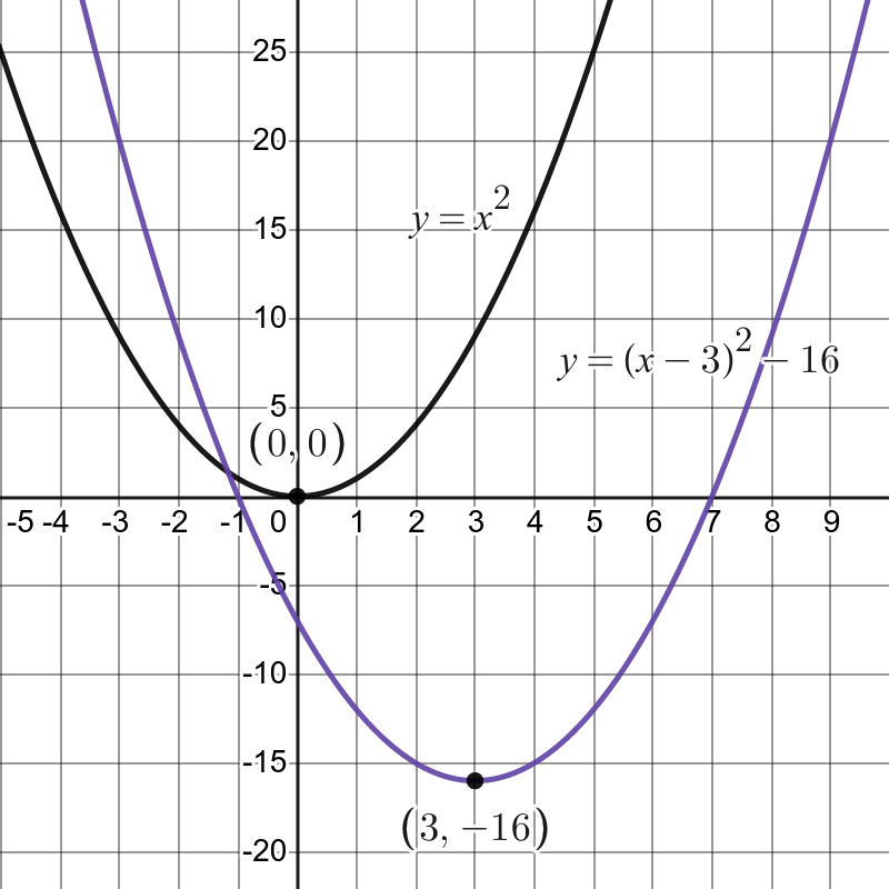
Figure 3.1: See the trough of the graph has been shifted right, and down

As seen in the graph above, the Completed Square format provided an easy way to find the minimum of a quadratic graph. It is in fact always true that the Completed Square format provides an easy way to find the minimum (or maximum²⁶) of the graph.

This is often extremely useful information when studying a real-world problem containing a quadratic formula.

Suppose we want to study the graph of \(y=Ax^2+Bx+C\). If we begin by completing the square and are able to write it in the format:

\[\begin{equation*} A\left(x+M\right)^2+N \end{equation*}\]

where \(M\) and \(N\) are numbers we have calculated then\(\ldots\)

the minimum (or maximum) of the graph will occur at \(x=-M\) and the value when \(x=-M\) will be \(y=N\).

In words, the minimum (or maximum) of the graph always occurs at the value of \(x\) which makes the bracket equal to zero.

Hence,

• horizontally, the graph’s trough (or peak) occurs when \(x+M=0\), i.e. \(x=-M\),
• vertically, the height of the graph at its trough (or peak) is \(0^2+N\), i.e. \(y=N\).

However, our real aim was to solve a quadratic equation²⁷, i.e. \(x^2-6x-7=0\) for this we still need to do a few short steps of algebra still.

\[\begin{align*} x^2 - 6x - 7 & = 0 && \text{became...} \\ (x-3)^2-16 & = 0 && \text{which becomes...} \\ (x-3)^2 & = 16 \\ \end{align*}\]

So our first step is to move the constant to the other side so that it says bracket squared equals constant.

Now we square root both sides… remembering that there are two square roots of every positive number, in this case \(+4\) and \(-4\) both square into \(16\).

So we get \[\begin{align*} (x-3) & = +4 \text{ or } -4, && \text{so...} \\ x = & +7 \text{ or } -1 \end{align*}\]

These general steps of algebra used here are the same every time you use completing the square.

Standard steps for the final equation solving part of completing the square:

• Move the constant to the right (i.e. add/subtract from both sides).
• Square-root both sides²⁸ (remembering there are two answers).
• Move the constant next to \(x\) to the right (i.e. add/subtract from both sides).
• You should be left with \(x\) as the subject.

In comparison to factorization, which only worked some of the time, this method works all the time. The times that factorization works are when the answers are nice and neat (generally integer) answers for \(x\). In general, however, you should expect your answers to a quadratic to contain surds (square root symbols). If the answer does involve surds, then factorization wasn’t the right approach to take. This completing the square method does get a little trickier if the starting equation doesn’t begin with \(1x^2\), so here’s a full typical example.

3.9.2 Completing the square: a typical difficult example

We are asked to solve

\[\begin{equation} 3x^2+2x-7 = 0 \tag{3.20} \end{equation}\]

We first need to get rid of the factor of \(3\), so we divide through by \(3\) (because we need \(1x^2\) on the front not \(3x^2\)) and get \[\begin{equation*} x^2+\frac{2}{3}x-\frac{7}{3} = 0 \end{equation*}\] Now we need to find half of the \(x\)-term, i.e. half of \(\frac{2}{3}\), which is \(\frac{1}{3}\) and form the squaring bracket. We want these two sides to balance: \[\begin{equation*} \left(x+\frac{1}{3}\right)^2+\text{Y}=x^2+\frac{2}{3}x-\frac{7}{3} \end{equation*}\] where we need to work out what value to place in for \(Y\). The \(x^2\) and \(x\) terms already match, by our clever construction, so it’s only the constant parts that need to be matched still²⁹.

The easiest way to find \(Y\) is just to copy the existing constant term down, and subtract off the extra final term you’ve introduced with your brackets expansion. i.e. \[\begin{equation*} \left(x+\frac{1}{3}\right)^2-\frac{7}{3}-\left(\frac{1}{3}\right)^2. \end{equation*}\] We have copied out the \(-\frac{7}{3}\) from the original, but we have introduced a \(\left(\frac{1}{3}\right)^2\) with our bracket, so we just subtract it off again.

The reason this works is because \[\begin{equation*} \left(x+\frac{1}{3}\right)^2 - \left(\frac{1}{3}\right)^2 = x^2+\frac{2}{3}x, \end{equation*}\] by subtracting off the square of the constant term in our bracket we just get the \(x^2\) and \(x\) terms.

So, \[\begin{align*} x^2 +\frac{2}{3}x-\frac{7}{3} & = \left(x+\frac{1}{3}\right)^2-\left(\frac{1}{3}\right)^2-\frac{7}{3} \\ & = \left(x+\frac{1}{3}\right)^2 - \frac{22}{9}, \end{align*}\] since \(-\frac{1}{9}-\frac{7}{3} = -\frac{1}{9}-\frac{21}{9} = -\frac{22}{9}\).

So we’ve turned our original equation (3.20) into \[\begin{equation} \left(x+\frac{1}{3}\right)^2-\frac{22}{9} = 0 \end{equation}\] The final steps are to make \(x\) the subject.

• We shall add \(\frac{22}{9}\) to be both sides, then
• Square root both sides (remember there are two answers)
• Subtract \(\frac{1}{3}\) from both sides to turn the left from \(x+\frac{1}{3}\) into just \(x\)

Let’s see these steps in action:

\[\begin{align*} \left(x+\frac{1}{3}\right)^2-\frac{22}{9} & = 0 \\ \left(x+\frac{1}{3}\right)^2 & =\frac{22}{9} \\ x+\frac{1}{3} & = +\sqrt{\frac{22}{9}} \text{ or } -\sqrt{\frac{22}{9}} \\ x & = +\sqrt{\frac{22}{9}}-\frac{1}{3} \text{ or } -\sqrt{\frac{22}{9}}-\frac{1}{3} \end{align*}\] These are our two answers for \(x\).

As mentioned at the start of this section, this method is a little more work than using the formula (see 3.10). In the long term it is worth knowing this method too, but do expect to make some algebraic errors when first trying to use it.

Here is a video demonstration of the method, for you to watch before attempting your own examples:

Alternative direct video link:

https://gcu.planetestream.com/View.aspx?id=5991~4y~AogxJYFc

Practice Complete the square for these six quadratic equations: \[ x^2 + 4x + 9 =0 \] \[ x^2 + 4x - 12 =0 \] \[ x^2 - 5x + \frac{1}{4} =0 \] \[ x^2 - 5x + 3 =0 \] \[ 2x^2 - 2x + 1 =0 \] \[ x^2 -x -1 =0 \]

Here are the six correct answers, in random order. Match your six answers up with these six formulae:

\[ \left(x-\frac{1}{2} \right)^2 + \frac{1}{4} = 0 \] \[ \left(x+2 \right)^2 + 5 = 0 \] \[ \left(x-\frac{5}{2} \right)^2- \frac{13}{4} = 0 \] \[ \left(x-\frac{1}{2} \right)^2 - \frac{5}{4} = 0 \] \[ \left(x-\frac{5}{2} \right)^2 - 6 = 0 \] \[ \left(x+2 \right)^2 -16 = 0 \]

Bonus question: Which of these problems has solutions of \(x=\frac{5}{2}+\sqrt{6}\), and \(x=\frac{5}{2}-\sqrt{6}\)?

3.10 The Quadratic formula

As explained in the Completing the Square section (3.9), the quadratic formula also always works. It has the advantage of being slightly faster, assuming you can remember the formula, and don’t mess up any of the algebra.

To use the quadratic formula you first need to put your problem into the standard format:

The standard quadratic equation format is \[\begin{equation} Ax^2+Bx+C=0 \tag{3.21} \end{equation}\] where \(A,B\) and \(C\) are constants to be identified.

Here are some examples for you to do and check your answers:

Quadratic equation	\(A\)	\(B\)	\(C\)
\(x^2-3x+2=0\)	1	-3	2
\(-x^2+x+7=0\)	-1	1	7
\(3x^2-x+1=0\)	3	-1	1
\(-5x^2+13=0\)	-5	0	13
\(x^2+4x=0\)	1	4	0

Once you’re comfortable with identifying \(A,B\) and \(C\) you can use the quadratic formula.

The Quadratic Formula says that the solutions to a standard format quadratic are: \[\begin{equation} x = \frac{-B \pm \sqrt{B^2-4AC}}{2A} \tag{3.22} \end{equation}\] where \(\pm\) means two answers, one with a \(+\) and the other with a \(-\).

Key points to note:

• It’s \(-B\) not \(+B\) at the start of the top of the fraction.
• The entire top of the fraction is divided by \(2A\) not just one of the parts.
• Take care with negative signs, especially in the \(-4AC\) part. If \(AC\) is negative then \(-4AC\) is positive.
• If \(B^2-4AC\) is negative, there will be no real solutions.³⁰ See Solubility Section 3.11 for further explanation.
• If \(B^2-4AC=0\) then both the \(\pm\) answers give the same answer, so there’s only one distinct answer for \(x\). It’s sometimes called a repeated solution.
• Many authors call the quantity \(B^2-4AC\) the discriminant of the quadratic equation.

So the full version of the two solutions are:

\[\begin{equation*} x = \frac{-B + \sqrt{B^2-4AC}}{2A}, \quad \text{and }\quad x = \frac{-B - \sqrt{B^2-4AC}}{2A} \end{equation*}\]

3.10.1 A simple example

Solve \(3x^2-x-1=0\) using the quadratic formula.

Answer: We identify \(A=3\), \(B=-1\) and \(C=-1\). So we substitute to get: \[\begin{equation*} x = \frac{--1 + \sqrt{(-1)^2-4\times 3\times -1}}{6}, \end{equation*}\] and also, \[\begin{equation*} x = \frac{--1 - \sqrt{(-1)^2-4\times 3\times -1}}{6} \end{equation*}\] which simplify into: \[\begin{equation*} x = \frac{1 + \sqrt{1+12}}{6}, \quad \text{and }\quad x = \frac{1 - \sqrt{1+12}}{6} \end{equation*}\] and finally into \[\begin{equation*} x = \frac{1 + \sqrt{13}}{6}, \quad \text{and }\quad x = \frac{1 - \sqrt{13}}{6} \end{equation*}\]

3.10.2 A video demonstration

Finally in this section, a short video demonstration of the use of the formula, with commentary.

Alternative direct video link: https://gcu.planetestream.com/View.aspx?id=3616~4q~qNPdenUP

Rather than provide more examples here, I suggest you search online for one of the many quadratic solving websites. It is good to get practice in how to search for ways to check your work, and many of them will also contain automated examples for you to try. At time of writing this link is a good example MathsIsFun.com

3.11 Solubility of quadratic equations

We discussed above that the method of factorization doesn’t always work, but that the other two methods do always work. However, what we mean by work is only that they will find the solutions if they exist.

When we attempt to solve a quadratic equation, we are trying to solve an equation that can first be re-arranged into our standard format as: \[\begin{equation*} Ax^2+Bx+C=0. \end{equation*}\] However, it’s quite easy to construct an example with no solutions at all. Just select \(A=1,\) \(B=0\) and \(C=1\) and we get \[\begin{equation*} x^2+1=0. \end{equation*}\] There are at least two ways to see that this equation has no solutions:

• \(x^2\), as a square, is never negative, so after adding \(1\) to it means the left-hand side of the equation cannot equal zero;
• The graph of \(y=x^2+1\) is U-shaped but never touches the \(x\)-axis. But the \(x\)-axis is where \(y=0\), i.e. \(x^2+1=0\)

Warning:

Not all quadratic equations have solutions. If the graph of \(y=Ax^2+Bx+C\) lies entirely above, or entirely below, the \(x\)-axis and never touches it, then there will be no values of \(x\) where \(Ax^2+Bx+C=0\). There are actually only three cases:

• The graph passes through the \(x\)-axis twice (this is typical);
• The trough/peak of the u-shaped/n-shaped graph exactly touches the \(x\)-axis (this is rare);
• The graph never goes through the \(x\)-axis (this is also fairly typical).

The first case, we get two solutions, and will be very typical of problems where you are asked to Solve or Find the solutions of.

The second case, you get one³¹ solution. This may also occur in examples you are given, an example would be \((x-1)^2=0\).

The third case, where there are no solutions³², is not that unusual but if you’re asked to find the solutions to a quadratic there is often an implicit implication that there are solutions to find. Similarly if the problem is derived from a real-life problem where solutions must exist, then this won’t happen.

The good news, is that it’s fairly easy to notice that you’re working with one of these cases with no solutions, as long as you are completing the square or using the quadratic formula.

When completing the square, you will know this no solutions case has occurred if at the late stage of square-rooting both sides the right hand side is negative and so cannot be square-rooted.

When using the quadratic formula, the quantity you square root is \(B^2-4AC\) (also called the discriminant in many notes). If this quantity is negative, then there will be no solutions.

If you know you’re being expected to find actual solutions, but your completing the square requires square-rooting a negative number; or your \(B^2-4AC\) is negative… then you have probably already made an algebraic mistake. Go back and carefully check your algebra.

3.12 Simultaneous linear equations

We have already seen linear equations, these were generally written in the format \(y=A+Bx\), for some constants \(A\) and \(B\). The word simultaneous refers to there being more than one equation, each of which needs to simultaneously³³ be true for a solution to be valid.

When solving simultaneous linear equations we generally start with a slightly different (but completely equivalent) display format, we move the unknown variables onto one side and put the constant on the other side. So rather than writing \(y=2x+1\) we write \(-2x+y=1\) or \(2x-y=-1\) both of which are the same and are just re-arrangements of the first. Two simultaneous equations might then look like this:

\[\begin{align} 2x - y & = -1 \tag{3.23} \end{align}\] \[\begin{align} x + 3y & = 24 \tag{3.24} \end{align}\]

To solve this pair of equations, we are looking for a pair of values \(x,y\) which simultaneously make both equations true. For example, \(x=2, y=5\), which we write \((x,y)=(2,5)\) solves (3.23) perfectly, because \(2\times 2-5 =-1\). However, this pair doesn’t solve (3.24) because \(2+3\times 5 = 17 \neq 24\). Trial-and-error is almost never a good idea for trying to solve such equations, because there are so many possibilities.

The solution which works for both (3.23) and (3.24) at the same time is \((x,y)=(3,7)\) but to find it will normally involve the use of one of the two standard techniques below:

• Elimination (Section 3.12.2), or
• Substitution (Section 3.12.3)

Before demonstrating the methods, we should first be totally clear what we mean by simultaneous equations.

The general format for a pair of simultaneous equations is written: \[\begin{alignat*}{2} Ax + By = E \\ Cx + Dy = F \end{alignat*}\] where \(A,B,C,D,E\) and \(F\) are all constants.

The unknown variables don’t need to be \(x\) and \(y\), but we just choose them as convenient letters. Similarly, although there are positive signs in the equations above, any variables could be negative which would override those signs. Furthermore, you can also generalize this problem to solve more than two simultaneous equations. However, with three (or more) unknowns both of these methods begin to take a long time and other more advanced techniques which use matrices are highly recommended.

Though beyond the scope of this chapter, you can (try and) solve any number of simultaneous equations as long as \[\begin{equation*} \text{The number of equations} = \text{The number of unknown variables} \end{equation*}\] For example, here are two problems with \(3\) and \(4\) unknowns respectively: \[\begin{align*} x+2y+5z & = 8 \\ 3x-y+z & = 3 \\ 3x +y -7z & = 12 \\ \end{align*}\] and \[\begin{align*} w+x+y+z &= 5 \\ 2w-x+3y-z &=-6 \\ -3w+x+2y-z &= -1 \\ 0.5w-2x+3y+4z &=6 \end{align*}\]

Much like when solving quadratic equations the answers in real-life are generally not nice round integers, although practice examples often are chosen in order to make the algebra fairly clean and so they do have integer answers. The example presented in (3.23) and (3.24) above was chosen to have a nice integer answer.

Warning: We shall solve this example by the two standard methods below, and the answers will be nice round integers. However, the ‘normal’ situation with solving simultaneous equations with real-life numbers results in answers which are just boring decimal numbers (or fractions) and not nice integers.

3.12.1 The geometrical intepretation

Returning now to two unknowns, which we’ll call \(x\) and \(y\)… before we dive into the main methods, a short geometrical interpretation.

Geometrical interpretation A linear equation in \(x\) and \(y\) actually describes all the points that make up a straight line on the standard \(x\) and \(y\) axes (i.e a graph).

So finding a pair of numbers \((x,y)\) which simultaneously solve two linear equations, means you’re finding co-ordinates \((x,y)\) which lie on both lines. So you’re actually finding the intersection of two lines.

3.12.2 The method of elimination

As the name suggests, the idea here is to eliminate something while solving the equations. The way this is done is by taking the two equations and adding or subtracting one from the other in a clever way to make one of the unknown letters cancel – and thus be eliminated.

We shall try and solve:

\[\begin{align} 2x - y & = -1 \tag{3.25} \end{align}\] \[\begin{align} x + 3y & = 24 \tag{3.26} \end{align}\]

It will be important to have labelled the equations so we can reference them in what follows.

There are two ways to do do this method,

• Either we choose to eliminate \(x\), or
• We choose to eliminate \(y\).

Either choice is fine, you normally just choose the one that will be easier to do, algebraically.

The idea is to add (or subtract) two equations together (adding the lefts and the rights) to form a new equation. If we do it immediately then both \(x\) and \(y\) will survive the process, on the left-hand-side. However, if we start by multiplying both sides of (3.25) by \(3\) then it turns into:

\[\begin{align} 6x - 3y & = -3 \tag{3.27} \end{align}\]

This equation is just an equivalent re-written version of (3.25)³⁴. However, we carefully chose to multiply by \(3\) because we can see it creates a \(-3y\) in (3.27) which will cancel with the \(+3y\) visible inside the other equation, (equation (3.26)).

So now we add together equations (3.26) and (3.27). This involves adding the left-hand-sides together and setting the answer equal to the sum of the right-hand-sides. We get:

\[\begin{align} \left(x + 3y\right)+\left(6x - 3y \right) & = \left(24\right)+\left(-3\right) \\ 7x & = 21 \end{align}\] Notice that the \(+3y-3y=0\) and \(24+(-3)=21\).

And we have reached a linear equation that mentions only \(x\) which can be solved by usual algebraic methods. In this case it’s very easy as we start with \(7x=21\) and dividing both sides by \(7\) immediately yields that \(x=3\).

This tell us that we need \(x=3\) to be true for both our original equations to be simultaneously true. But what about \(y\)? We can just use any of the equations to find the \(y\) which works with \(x=3\). All equations we use should give the same accompanying \(y\), which in this case yields \(y=7\) and our only solution is \[\begin{equation*} \left(x,y\right) = \left(3,7 \right). \end{equation*}\]

Alternatively, we could have chosen to eliminate \(x\) rather than \(y\). In this case we notice that it appears as \(+2x\) in (3.25) and as \(x\) in (3.26).

The clever step here would be to take the second equation, (3.26), and multiply both sides by \(2\) to create a new equation that also contains \(2x\).

However, now since both \(x\) terms are the same (and not the negative of each other as with the \(y\) example above) we should then subtract one equation from the other. Then the \(x\) terms will disappear from the next equation. You should try this yourself and see if you discover that \(y=7\) immediately.

In both these examples it was possible to leave one equation alone and multiply the other to get ready for the addition/subtraction. In more complicated examples you might need to multiply both equations by something to get two equations with matching \(x\) or \(y\) terms.

3.12.3 The method of substitution

This method requires less thinking than the elimination method. In the elimination method we needed to make a clever choice for the multiplication of one equation, to ensure one of the variables cancelled when we then added or subtracted our equations.

In contrast, with substitution, such thought isn’t required. However, the resulting calculations normally involve fractions or messier algebra.

With substitution the idea is as follows:

• Start with two equations as usual.
• Select one unknown variable, and one equation (which mentions it).
• Re-arrange the chosen equation to make the chosen variable the subject.
• Substitute the formula for your chosen variable into the other equation.
• Re-arrange and solve the for the variable you didn’t select.

The first couple of steps above, do involve a choice, and with practice you might develop the skills to select the easier route³⁵. But which variable and equation works most easily will depend upon the question and can be hard to predict.

We shall use the method to solve the same problem again:

\[\begin{align} 2x - y & = -1 \tag{3.28} \end{align}\] \[\begin{align} x + 3y & = 24 \tag{3.29} \end{align}\]

An easy choice is not difficult to spot here. We want to pick a variable and an equation then make our chosen variable the subject of our equation.

We choose the second equation ((3.29)) and the variable \(x\). This is easy because it requires very little algebra to make \(x\) the subject. We begin with \(x+3y=24\) and just need to subtract \(3y\) from both sides to move the \(3y\) to the other side and reach: \[\begin{align} x & = 24-3y \tag{3.30} \end{align}\]

We now have a formula for our chosen variable, \(x\), which we substitute into the other equation ((3.28)). By substitute we mean to use our known value of \(x\) (we just read the right-hand-side of (3.30)) inside the first equation.

Here is the result of the substitution and simplifying algebra:

\[\begin{align*} 2x - y & = -1 \\ 2\left(24-3y\right)-y & = -1 \\ 48-7y & = -1 \\ 48 & = -1+7y \\ 49 & = 7y \\ 7& = y \end{align*}\]

We replaced/substituted \(x\) with \(24-3y\) because we know they are equal. Then proceeded with standard algebra steps to make \(y\) the subject. Resulting in the discovery that \(y=7\) is the answer.

As in the method of elimination this gives us the value of one unknown variable, and we can use any of our equations to find the value of the other variable. In this case you can quickly discover when \(y=7\) that \(x=3\) and we obtain the same answer as previously.

Alternatively, a messier route tries to make \(y\) the subject of (3.29). The re-arrangement gives \[\begin{equation*} y = \frac{24-x}{3}. \end{equation*}\]

This can be substituted into the other equation: with \(2x-y=-1\) becoming \[\begin{equation*} 2x-\left(\frac{24-x}{3}\right) = -1 \end{equation*}\] but then the algebra required here to re-arrange and discover \(x=3\) is a fair bit messier. If you can avoid introducing fractions then it’s definitely recommended, but not always possible.

There are two other combinations of subject variable and equation we could have made.

You could of course make \(y\) the subject of (3.28) and the calculation would be straightforward.

However, making \(x\) the subject of (3.28) leads to another messy calculation.

3.12.4 Special cases

This isn’t quite the end of the story for simultaneous equations. When following either of the methods above there are two unexpected things that can happen. When you are re-arranging an equation to make a variable, say \(x\), the subject either of these events could happen:

1. All the \(x\)-terms might cancel, and you reach a totally factual equation like \(4=4\) or \(0=0\),
2. All the \(x\)-terms might cancel, and you reach a totally incorrect equation like \(4=2\) or \(1=0\).

Both of these can occur³⁶.

In Case 1 above, you’ve reached an equation that works for any and all \(x\) so there are solutions for every \(x\)! There will be infinitely many answers. Geometrically (see Section 3.12.1) you will have started with two equations describing exactly the same line, so all points on the line solve both equations!

In Case 2 above, you’ve reached an equation for which there are no \(x\) values that can make it true. So there are no answers that work for \(x\)! Geometrically (see Section 3.12.1) you will have started with two parallel lines which never meet each other. There will be no simultaneous solutions to your two equations.

Here’s a video to illustrate Case 1 (above) occurring:

Alternative direct video link:

https://gcu.planetestream.com/View.aspx?id=5992~4z~aYw9tYQz

Here’s a very similar video, but this time it’s Case 2 that occurs:

Alternative direct video link:

https://gcu.planetestream.com/View.aspx?id=5993~4A~CLLKdXaJ

Here’s is a random example to test yourself, you can click to try another different question after answering. I suggest you try both methods separately to see which one you prefer.

Link to Numbas on the web

In addition I recommend you look online for nice simultaneous equations solvers which can show you worked solutions to problems you try. At time of writing, this is a nice example: equationcalc.com

Finally some advanced examples, again you can randomize and get a new question via the link.

[Link to Numbas on the web](https://numbas.mathcentre.ac.uk/question/114447/advanced-simultaneous/embed/?token=0578e3c1-2599-47a3-9b3d-ae0b5cafd7df

3.13 Further practice exercises

For most topics in algebra the best way to learn and improve is through practice. So you are recommended to seek out your own further exercises.

However, there is also a specific further exercises section at the end of the notes here: Section 6.

3.14 Summary of chapter

Having worked through this chapter and attempted the exercises you should now have understanding of the following topics:

• Develop confidence working with basic operations, brackets, powers and grouping terms;
• Work with exponential and logarithm functions, including knowledge of the log laws;
• Develop confidence using algebra to simplify and solve equations, including the use of operation inverses;
• Be able to identify a quadratic equation and be able to use:
  • Factorization,
  • Completing the square, or
  • The Quadratic Formula to solve them; and
• Be able to solve simultaneous linear equations by elimination and substitution methods.