5 Introduction to Matrices

A matrix is just a collection of numbers arranged into a grid. They are always drawn with brackets⁶⁷ around them. Here are a few examples of matrices⁶⁸ of different shapes and sizes,

\[\begin{equation} \begin{pmatrix}4 & 0 & 3 & -1 \end{pmatrix},\; \begin{pmatrix}1 & \sqrt{2} \\ y & 7 \end{pmatrix},\; \begin{pmatrix}3 & 9 \\ -1 & 7 \\ 0 & 3.4 \end{pmatrix},\; \begin{pmatrix}4 & 5 & 5 \\ 1 & -2 & -9 \\ 1 & 0 & 0 \end{pmatrix}. \tag{5.1} \end{equation}\]

In this introduction most of the numbers in the matrix grid will be integers, to make your calculations easier, but they don’t need to be. As you can see above you can even just insert algebra letters, to represent unknowns.

Matrices have a very wide range of practical uses, here are just a few you may come across:

For representing movements and performing calculations in computer graphics;
For representing mechanical systems and movements;
For representing electrical circuits and calculating currents and voltages;
For storing, then manipulating statistical data;
As a large family of objects useful in cryptography;
For representing data in, and then solving, business optimization problems.

The two data applications above both hint at the use of spreadsheet software, which naturally contains boxes in a grid formation for storing numbers.

We have actually seen matrices before, when we discussed the Rectangular/Cartesian format for vectors. In 4.3 we introduced a notation which placed the components of a vector into a column inside parentheses as follows:

\[ \underline{v} = \begin{pmatrix}3 \\ -3 \\ 7 \end{pmatrix}. \]

This format is just a special case of a matrix with grid of width \(1\) and height \(3\).

Fundamentally matrices are just a clever notation for holding many numbers in a grid format at the same time. However, as with lots of notation in maths, once we have a nice notation if we invent nice ways to manipulate it and do algebra then we can later make solving very complex problems relatively easy. We shall see exactly this for solving systems of linear equations later (i.e. solving simultaneous equations in Sections 5.6, 5.7 and 5.8).

5.1 Terminology

In absolute consistency with the notation used with vectors, the numbers in a matrix can be described by which row and which column they lie in. In keeping with terminology for vectors, rows are horizontal and columns are vertical.

A matrix can therefore be thought of as a collection of rows stacked on top of each other, or as a collection of columns placed side-by-side.

5.1.1 Describing the shape of a matrix

When it comes to describing the shape we just need to tell the reader how many rows and how many columns the matrix has. Note that matrices are always a full grid, every row is the same length and every column is the same length (height).

Formal shape definition

A matrix with \(3\) rows and \(2\) columns is called a \(3\)-by-\(2\) matrix, or a \((3\times 2)\) matrix.

In general, if it has \(m\) rows and \(n\) columns then it is called an \(m\)-by-\(n\) matrix.

Notice that the order of \(m\) and \(n\) will matter⁶⁹ so it’s important to agree which number comes first, and which second.

The same memory aids exist here remembering the usage of rows and columns, from when we discussed vectors.

fiRst = Rows

seCond = Columns

Additionally, for anyone who confuses the meanings of rows and columns\(\ldots\) seats in cinemas are arranged in rows, and good old Roman columns on buildings stand vertically.

This \(m\)-by-\(n\) notation will be important if we use a letter like \(M\) in algebra to describe a matrix, because you cannot tell from just the letter \(M\) what shape it is. Naturally if you have written out the matrix in full inside brackets then it will be obvious what shape it is!

5.1.2 Describing elements of a matrix

If we wish to refer to a specific number inside a matrix, we can identify it by which intersection of row and column it lies at.

For example, in this large matrix,

\[ M = \begin{pmatrix}3 & 1 & 8 & -1 \\ 2 & 3 & \color{red}{0} & 9 \\ 3 & -7 & 5 & 9 \end{pmatrix}\]

the element at row \(2\), column \(3\) is a \(0\) (zero)⁷⁰.

In repeated consistency with the previous section, we can shorten the description of the element in Row 2 and in Column 3, and just say that the \((2,3)\) element of the matrix is \(0\).

Various authors of books may also describe elements of a matrix as entries. Additionally the \((2,3)\) element of \(M\) can also be called \(M(2,3)\) or \(M_{2,3}\) or even \(m_{23}.\) This last notation without a comma is only safe if the number of rows and columns is small, otherwise you might not be able to tell where the two numbers separate.

5.1.3 Comparing matrices

In most work with matrices we generally only deal with one (or two) different shapes within a single question. Indeed a lot of the most interesting uses of matrices are specific to what we shall later call square matrices (which have the same number of rows as they have columns).

When it comes to directly comparing two matrices, we only say that two matrices are equal if they are exactly the same shape and all the elements match exactly.

Before we conclude this terminology section, a few exercises to provide you with some practice with the new terms.

Link to Numbas on the web

Question 1: For each of the matrices in the original list in this chapter (see (5.1)) identify what shape they are in the \(m\)-by-\(n\) notation.

Question 2: Were any pair of the matrices in those examples the same shape as each other?

Question 3: Finally, what shape is this matrix and what is its \((1,4)\) element?

\[ \begin{pmatrix}4&-7&9&8 \\ 0&91&-3&-1 \\ 2&5&7&2 \\ 1&2&16&-3\end{pmatrix}\]

Answers:

Question 1⁷¹

Question 2⁷²

Question 3⁷³

5.2 Algebra operations

Whenever we introduce a new mathematical object, such as a matrix, we need to also check whether the standard algebra we do with numbers can be applied to it too. Sometimes new mathematical objects require special meanings for addition, multiplication, division, etc… However, the good news is that for matrices the basic rules are very similar. The main complication occurs in the same place as it did with vectors. Namely, that when we think about multiplication there are two choices: do we want to multiply by a scalar or by another matrix? We shall see the answers later.

As with all new objects the idea is to define how to do algebra in the most sensible way so that we can continue to perform as much of our normal algebra as possible.

5.2.1 Adding and subtracting matrices

These calculations are going to be nice and straightforward.

First a couple of warnings\(\ldots\)

Some things you cannot do:

You cannot add a single number to a matrix so \(4 + \begin{pmatrix}2 & -3 \\ 1 & 5 \end{pmatrix}\) doesn’t make sense.
You cannot add two matrices if they are not exactly the same shape.

Now for the good news, once you have two matrices of identical shape, adding them together is as easy as just separately adding every element with its matching position element in the other matrix. Subtraction is the same, you just subtract the second matrix elements from the first, one-by-one. Let’s see one example of each, after which is should be very obvious how it works.

To add two matrices they need to be the same shape, and then you add together corresponding location elements like this:

\[\begin{align*} \begin{pmatrix}1 & 4 \\ -1 & 0 \\ 3 & 1 \\ 4 & -1 \end{pmatrix}+ \begin{pmatrix}4 & 2 \\ 1 & -4 \\ 9 & -5 \\ 1 & 0 \end{pmatrix}& = \begin{pmatrix}1+4 & 4+2 \\ -1+1 & 0+-4 \\ 3+9 & 1+-5 \\ 4+1 & -1+0 \end{pmatrix}\\ & = \begin{pmatrix}5 & 6 \\ 0 & -4 \\ 12 & -4 \\ 5 & -1 \end{pmatrix} \end{align*}\]

Eight separate additions were performed, check them!

To subtract one matrix from another it’s the same idea. They need to be the same shape, and you just need to make sure you know which number is on the left and which on the right:

\[\begin{align*} \begin{pmatrix}7 & -4 \\ 2 & 4 \end{pmatrix}- \begin{pmatrix}1 & -3 \\ -5 & 6 \end{pmatrix}& = \begin{pmatrix}7-1 & -4--3 \\ 2--5 & 4-6 \end{pmatrix}\\ & = \begin{pmatrix}6 & -1 \\ 7 & -2 \end{pmatrix} \end{align*}\] Here four separate standard subtractions were performed, check them!

5.2.2 Scalar multiplication of matrices

Also relatively easy is the idea of multiplying a whole matrix by a number⁷⁴. For this calculation you just multiply every element of the matrix by this number. If \(M\) is a matrix, you can then talk about \(2M\), and \(3M\) and \(kM\) for any constant \(k\).

Let’s see an example combining addition and multiplication by a scalar.

Let \(M=\begin{pmatrix}1 & 4 \\ 0 & 3\end{pmatrix}\) and \(N=\begin{pmatrix}-2 & 3 \\ 1 & -5\end{pmatrix}\) both be \(2\)-by-\(2\) matrices.

First let’s calculate \(3M\):

\[ 3M = 3\begin{pmatrix}1 & 4 \\ 0 & 3\end{pmatrix}= \begin{pmatrix}3 & 12 \\ 0 & 9\end{pmatrix}\]

You should check each element matches what you were expecting.

Now for a linear combination of \(M\) and \(N\), let’s calculate \(3M-2N\):

\[\begin{align*} 3M-2N = \begin{pmatrix}3 & 12 \\ 0 & 9\end{pmatrix}- 2\begin{pmatrix}-2 & 3 \\ 1 & -5\end{pmatrix}\\ & = \begin{pmatrix}3 & 12 \\ 0 & 9\end{pmatrix}- \begin{pmatrix}-4 & 6 \\ 2 & -10\end{pmatrix}\\ & = \begin{pmatrix}7 & 6 \\ -2 & 19\end{pmatrix} \end{align*}\] Again, check the calculations here to convince yourself you know what’s happening.

Link to Numbas on the web

5.2.3 Matrix multiplication using the Scalar product

As forewarned, multiplying a matrix by another matrix (known as matrix multiplication) is the most complicated part of working with matrices. We want a way of multiplying matrices by each other which has practical applications and is useful. The good news is that there is indeed a way to do this which is extremely useful in many applications.

The bad news is that the process involves a lot more calculations than the other algebra seen so far. None of the calculations are complex, but there are quite a lot of them. Conveniently if you have already studied the Scalar Product⁷⁵ of two vectors (see 4.10) then the method can be understood more easily.

So first we shall remind ourselves how the Scalar Product of two vectors of the same shape works. Remember first that a vector is just a matrix with \(1\) column.

Scalar Product definition (reminder)

If we have two vectors of the same shape (i.e. they have the same number of elements) then their Scalar Product is calculated by

Multiplying each element of one vector by the element of the other vector in the corresponding position, then
Adding together all these answers.

Here’s the example we saw before,

For vectors \(\underline{v}=\begin{pmatrix}8\\-2 \end{pmatrix}\) and \(\underline{w}=\begin{pmatrix}3\\4 \end{pmatrix}\) their Scalar Product is

\[ \underline{v}\cdot\underline{w} = \begin{pmatrix}8\\-2 \end{pmatrix} \cdot \begin{pmatrix}3\\4 \end{pmatrix}= 8 \times 3 + (-2)\times 4 = 16. \]

As an example for 3-dimensional vectors, \(\underline{v}=\begin{pmatrix}2\\-1\\4 \end{pmatrix}\) and \(\underline{w}=\begin{pmatrix}5\\8\\-1 \end{pmatrix}\) their Scalar Product is

\[\begin{align*} \underline{v}\cdot\underline{w} & = \begin{pmatrix}2\\-1\\4 \end{pmatrix} \cdot \begin{pmatrix}5\\8\\-1 \end{pmatrix}, \\ & = 2 \times 5 + (-1)\times 8 + 4 \times (-1),\\ & = 10-8-4=-2. \end{align*}\]

It was worth seeing this Scalar Product definition (again) because our method for finding the product of two matrices is actually just going to be a collection of different Scalar Products! In words, the product of two matrices (called \(A\) and \(B\)), is going to be a new matrix whose elements are the separate Scalar Products created by matching every row from \(A\) with every column from \(B\). First a couple of warnings…

Warning 1:

When multiplying matrices together the order matters, so \(A \times B\) and \(B \times A\) are different calculations⁷⁶

Warning 2:

Two matrices \(A\) and \(B\) can only be multiplied together to create \(AB\) if …

“The number of columns of \(A\)” equals “The number of rows of \(B\).”

Example

We consider the product of two matrices, called \(A\) and \(B\), which are defined as follows \[ A = \begin{pmatrix}1 & 2 & 3 \\ 4 & 5 & 6 \\ 7 & 8 & 9 \end{pmatrix}\] and \[ B = \begin{pmatrix}11 & 2 \\ 4 & 5 \\ 7 & 8 \end{pmatrix}\] The product \[AB\] is created by writing \(A\) to the left of \(B\)⁷⁷ \[ AB = \begin{pmatrix}1 & 2 & 3 \\ 4 & 5 & 6 \\ 7 & 8 & 9 \end{pmatrix}\begin{pmatrix}11 & 2 \\ 4 & 5 \\ 7 & 8 \end{pmatrix}\]

Notice that the length of each row of \(A\)⁷⁸ matches the height of each column of \(B\)⁷⁹. Both of these quantities are equal to \(3\).

This is how we start to write the product of two matrices \(A\) and \(B\). But how about the method for actually calculating the product? Well in words, we have to do the following…

To calculate the product of two matrices involves lots of separate calculations:

One calculation for every combination using… a row from \(A\) and a column from \(B\)!
In our example above \(A\) has \(3\) rows, so there are \(3\) row choices.
In our example above \(B\) has \(2\) columns, so there are \(2\) column choices.
Together this means there are \(3\times 2 = 6\) combinations of row and column choices. For completeness we shall list them all here:

Row 1 (of \(A\)) with Column 1 (of \(B\))
Row 1 (of \(A\)) with Column 2 (of \(B\))
Row 2 (of \(A\)) with Column 1 (of \(B\))
Row 2 (of \(A\)) with Column 2 (of \(B\))
Row 3 (of \(A\)) with Column 1 (of \(B\))
Row 3 (of \(A\)) with Column 2 (of \(B\))

You will need to systematically go through all 6 combinations to calculate the product \(AB\). You are creating the entries for \(AB\) one at a time.

For every (row from \(A\),column from \(B\))-pair you need to calculate the Scalar Product. You insert the answer in the corresponding position in the answer matrix. i.e. if you used Row \(i\) (of \(A\)) and Column \(j\) (of \(B\)) then their Scalar Product should be inserted in Row \(i\), Column \(j\) of the product \(AB\).

We’ll write out the formal definition in words, and set an exercise for you to try, then do a fully worked example. The example will likely make more sense than the wordy definition when you first read it.

Definition of matrix multiplication

Once you have selected a row from \(A\) and a column from \(B\) you treat them both as vectors of the same length and find their Scalar Product.

The answer to multiplying two matrices together is another matrix, and the answer has shape⁸⁰ which matches the number of rows of \(A\) and the number of columns of \(B\). In this case \(A\) had 3 rows and \(B\) had 2 columns, so \(AB\) has 3 rows and 2 columns. This will become much clearer when we learn what to do with the Scalar Products explained above.

For each row of \(A\) and for each column of \(B\) you find the Scalar Product of those vectors and put the answer in the location described by where you got the vectors from!

So, using Row 3 of \(A\) and Column 1 of \(B\) means you calculate this Scalar Product \[\begin{pmatrix}7 \\ 8 \\ 9 \end{pmatrix}\cdot \begin{pmatrix}11 \\ 4 \\ 7 \end{pmatrix}= 77+32+63 = 172\] and the answer of \(172\) is placed in Row 3, Column 1 of the answer, i.e. in \(AB\) it appears like this \[AB = \begin{pmatrix}\cdot & \cdot \\ \cdot & \cdot \\ 172 & \cdot \end{pmatrix}. \]

Note: We rotated Row 3 of \(A\) so we could write it next to Column 1 of \(B\) to do the Scalar Product.

Practice

Using the method outlined above try and calculate the five missing values in \(AB\) (represented by dots) here: \[AB = \begin{pmatrix}\cdot & \cdot \\ \cdot & \cdot \\ 172 & \cdot \end{pmatrix}\]

As a reminder here are \(A\) and \(B\) in this example: \[ A = \begin{pmatrix}1 & 2 & 3 \\ 4 & 5 & 6 \\ 7 & 8 & 9 \end{pmatrix}, \quad B = \begin{pmatrix}11 & 2 \\ 4 & 5 \\ 7 & 8 \end{pmatrix}\]

Hint: to find the Row 1, Column 2 entry of \(AB\), you need to find the Scalar Product of Row 1 from \(A\) with Column 2 from \(B\).⁸¹

It’s strongly recommended that you watch this video to see matrix multiplication in action:

Alternative direct video link: https://gcu.planetestream.com/View.aspx?id=5555~4u~vB7eUMN3

It is often easier to remember this method by seeing the rows and columns highlighted, so let’s look at another example. Imagine we want to find the following matrix product:

\[ \begin{pmatrix}8 & 1 & 3 & -2 \\ 4 & 0 & -6 & 1 \end{pmatrix}\begin{pmatrix}3 & 1 & 2 \\ -1 & 2 & 3 \\ 0 & 5 & -4 \\ 2 & 0 & -2 \end{pmatrix} \]

We begin by highlighting Row 1 of \(A\) with Column 1 of \(B\), the result from finding the Scalar Product of these two highlighted vectors will go into Row 1, Column 1 of our answer:

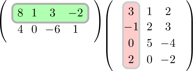
Figure 5.1: Highlighted rows and columns for matrix multiplication

This Scalar Product has value \(8 \times 3+1\times (-1)+3\times 0 +(-2)\times 2 = 19\).

Next we highlight Row 1 of \(A\) with Column 2 of \(B\), the result from finding the Scalar Product of these two highlighted vectors will go into Row 1, Column 2 of our answer:

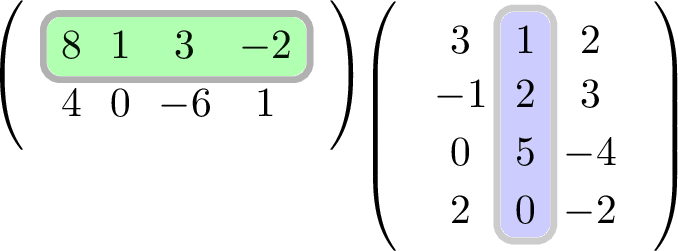
Figure 5.2: Highlighted rows and columns for matrix multiplication

This Scalar Product has value \(8 \times 1+1\times 2+3\times 5 +(-2)\times 0 = 25\).

Finally we highlight Row 1 of \(A\) with Column 3 of \(B\), the result from finding the Scalar Product of these two highlighted vectors will go into Row 1, Column 3 of our answer:

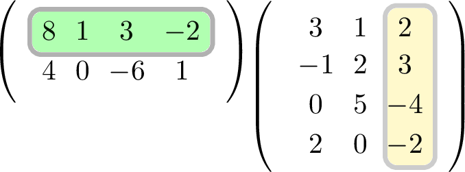
Figure 5.3: Highlighted rows and columns for matrix multiplication

This Scalar Product has value \(8 \times 2+1\times 3+3\times (-4) +(-2)\times (-2) = 11\).

These three calculations give (Row 1, Column 1), then (Row 1, Column 2) and (Row 1, Column 3) of the answer. We still need to repeat the above procedure but using Row 2 of \(A\) each time to find Row 2 values in our answer.

Practice

Calculate the three Scalar Products in the coloured images above, and then repeat the process but using Row 2 of \(A\) each time. Insert your six answers into their correct places to obtain your end result: the matrix product \(AB\).

Verify that you get the following answer:

\[ \begin{pmatrix}8 & 1 & 3 & -2 \\ 4 & 0 & -6 & 1 \end{pmatrix}\begin{pmatrix}3 & 1 & 2 \\ -1 & 2 & 3 \\ 0 & 5 & -4 \\ 2 & 0 & -2 \end{pmatrix}= \begin{pmatrix}19 & 25 & 11 \\ 14 & -26 & 30 \end{pmatrix} \]

If you get a different value in any element, go back and repeat the product. It is very common to make numerical mistakes when calculating matrix products.

When introducing matrix multiplication it was mentioned that you need each row of \(A\) to be of the same length as each column of \(B\), this is actually not something you need to remember if you know the method! Notice that it would have been impossible to calculate the Scalar Products above unless every row of \(A\) matched each column of \(B\) for length!

A tip and a warning

If the two matrices match the correct shape requirement above then you can find the product using the method outlined.

If they don’t match this shape requirement then you cannot multiply the matrices together.

Warning: The order of the matrix product matters! Which matrix was written on the left and which on the right will effect the answer. In fact it may not even be possible(!) to multiply the matrices, and even if you can you will normally get a totally different answer! So always make sure you know which matrix appears first in the product.

Link to Numbas on the web

In the examples provided above you were asked to perform matrix multiplications of matrices that were selected to have the correct shapes to make matrix multiplication possible. As a small exercise in checking what shape matrices can actually be multiplied together, here are a few examples to think about.

Here are three matrices, \(A\), \(B\) and \(C\):

\[ A = \begin{pmatrix}1 & 4 \\ 0 & -1 \end{pmatrix},\quad B=\begin{pmatrix}4 \\ 7 \\ 2 \end{pmatrix},\quad C = \begin{pmatrix}3 & 2 & -4 \\ 0 & 1 & 1 \end{pmatrix} \]

Question: Which of the six matrix products \(AB\), \(AC\), \(BC\), \(BA\), \(CA\) and \(CB\) are actually possible?

If unsure, then refer back to the definition of matrix multiplication to think about what Scalar Products you need to calculate.

Hint: The length of each row in the left matrix, needs to match the length of each column in the right matrix.

Answers:⁸²

5.3 Special matrices, quantities and procedures

Matrices are a very rich area of maths, there are so many different matrices with so many uses that there are a few certain shapes and specific matrices which are given special names because they come up in numerous applications…

5.3.1 General pattern: Square matrices

A matrix is described as square if the number of rows matches the number of columns. The shape of the matrix grid will look like a square, it’s as simple as that! Here are some examples of square matrices, of different sizes

\[ \begin{pmatrix}1 & 6 \\ -4 & -123 \end{pmatrix},\quad \begin{pmatrix}5 & 0 & 1 \\ 1 & 2 & 0 \\ -1 & 2 & 0 \end{pmatrix}, \quad \begin{pmatrix}7 & 6 & -1 & 0 \\ 1 & -1 & 2 & 9 \\ 0 & 3 & -4 & 9 \\ 0 & 0 & 1 & 2 \end{pmatrix}. \]

5.3.2 Special matrix: the zero matrix

There isn’t just one zero-matrix, there is in fact one zero-matrix for every given possible matrix shape. Perhaps unsurprisingly the zero matrix of a particular shape is just a matrix where every element is a zero. e.g. \[ Z = \begin{pmatrix}0 & 0 & 0 & 0 & 0 \\ 0 & 0 & 0 & 0 & 0 \\ 0 & 0 & 0 & 0 & 0 \end{pmatrix}, \textrm{ or } Z=\begin{pmatrix}0 & 0 \\ 0 & 0 \end{pmatrix}. \]

This matrix behaves a lot like the number \(0\) when used in matrix addition. Just like adding zero to a number makes no difference to a number, adding the zero matrix to a matrix makes no difference to the matrix.

5.3.3 Special matrix: the identity matrix – (see inverses later)

More useful than the zero matrix is the identity matrix, it is like the zero matrix above, but useful when doing matrix multiplication. The identity matrix can be described in three steps:

it has to be a square matrix (see 5.3.1);
all the elements along the diagonal from the top left to the bottom right are ones; and
all the other elements are zeros.

So here are the identity matrices of shapes \(2\)-by-\(2\), \(3\)-by-\(3\) and \(4\)-by-\(4\) :

\[\begin{equation} \begin{pmatrix}1 & 0 \\ 0 & 1 \end{pmatrix}, \quad \begin{pmatrix}1 & 0 & 0 \\ 0 & 1 & 0 \\ 0 & 0 & 1 \end{pmatrix}, \quad \begin{pmatrix}1 & 0 & 0 & 0 \\ 0 & 1 & 0 & 0 \\ 0 & 0 & 1 & 0 \\ 0 & 0 & 0 & 1 \end{pmatrix} \tag{5.2} \end{equation}\]

The reason they are called identity matrices comes from the use of the word identity when describing the ordinary multiplication of a number by \(1\). The number \(1\) has the property that when you multiply a number by it then nothing changes, e.g. \(13\times 1=13\) and \(1 \times x = x\).⁸³ So while the zero matrix made no difference when adding (see 5.3.2), the idea with the identity matrix is the following:

Multiplying a matrix by an identity matrix leaves it unchanged

Just like multiplying a number by \(1\) makes no difference to the number, multiplying a matrix by the identity matrix makes no difference to the matrix!

This is less easy to see, but you should definitely try the following calculation for yourself:

\[ \begin{pmatrix}3 & 1 & -1 \\ 8 & -2 & 4 \end{pmatrix}\begin{pmatrix}1 & 0 & 0 \\ 0 & 1 & 0 \\ 0 & 0 & 1 \end{pmatrix}= \begin{pmatrix}3 & 1 & -1 \\ 8 & -2 & 4 \end{pmatrix}\]

In algebra an identity matrix is represented by an \(I\) (a capital \(i\)), so the product above is written as \(MI = M\). We say that for any matrix \(M\), multiplying it by \(I\) (of the correct shape) gives you back \(M\). If \(M\) is a square matrix, then you can easily check that also \(IM=M\), so that you can put \(I\) on the left or the right of \(M\) and get the same answer. This property that \(MI=IM\) is very special to an identity matrix \(I\), because normally changing the order of the product of two matrices will give a totally different answer.

Note that we had to select an identity matrix of the correct size for the matrix multiplication to make sense. In this example we had to choose a matrix whose columns were length \(3\) to match with the length of each row of our starting matrix.

When working with identity matrices and algebra we normally use the letter \(I\) to describe the matrices, so the standard names of the matrices in (5.2) are actually \[ I_2 = \begin{pmatrix}1 & 0 \\ 0 & 1 \end{pmatrix}, \quad I_3=\begin{pmatrix}1 & 0 & 0 \\ 0 & 1 & 0 \\ 0 & 0 & 1 \end{pmatrix}, \quad I_4=\begin{pmatrix}1 & 0 & 0 & 0 \\ 0 & 1 & 0 & 0 \\ 0 & 0 & 1 & 0 \\ 0 & 0 & 0 & 1 \end{pmatrix}. \]

5.3.4 Special matrix: the transpose (and how to create it)

This one isn’t quite a special matrix like the zero and identity matrices were, but it falls into the same category. Transposing is actually a procedure, something you can do to a matrix. To find the transpose of a matrix you just need to swap all the rows and columns.

The shape of the matrix will transform from an \(m\)-by-\(n\) matrix into an \(n\)-by-\(m\) matrix. e.g.

\[ \begin{pmatrix}1 & 8 & 0 \\ -1 & 3 & -5 \end{pmatrix}\text{ becomes } \begin{pmatrix}1 & -1 \\ 8 & 3 \\ 0 & -5 \end{pmatrix}, \]

i.e. Row \(1\) became Column \(1\), and Row \(2\) became Column \(2\). So our \(2\)-by-\(3\) matrix became a \(3\)-by-\(2\) matrix.

Interestingly the transpose of a square matrix will be another square matrix of the same shape.

Authors will use the letter \(T\) in a superscript as notation for the transpose of a matrix. So \(M\) becomes \(M^T\), e.g. \[ \begin{pmatrix}5 & 0 & 2 \\ 1 & -3 & 99 \\ 4 & 0 & 2 \end{pmatrix}^T = \begin{pmatrix}5 & 1 & 4 \\ 0 & -3 & 0 \\ 2 & 99 & 2 \end{pmatrix}\]

An often useful fact about transposes is that if you transpose twice you will get back to where you started. It’s true for any matrix \(M\) that \[ (M^T)^T = M.\] Check it for yourself in the examples above.

You will also note that all the identity matrices (see Section 5.3.3) are unaffected by finding their transpose. e.g.

\[ \begin{pmatrix}1 & 0 & 0 \\ 0 & 1 & 0 \\ 0 & 0 & 1 \end{pmatrix}^T = \begin{pmatrix}1 & 0 & 0 \\ 0 & 1 & 0 \\ 0 & 0 & 1 \end{pmatrix}, \text{ i.e. }I_3^T = I_3 \]

5.3.5 General pattern: Diagonal matrices

Like with identity matrices, we shall also use the adjective diagonal for square matrices. When describing identity matrices, every single element of the matrix was specified, either as a \(1\) (along the Northwest to Southeast diagonal), or a \(0\) elsewhere. We shall talk about that same diagonal from top left to bottom right when introducing diagonal matrices, but not every element will have a specified value.

A square matrix is called diagonal if *all the elements not on the diagonal from top left to bottom right are zero**. This definition may feel like a negative way of describing something, so an alternative more constructive description would be as follows:

In a diagonal matrix you can choose any values for the elements along the Northwest-to-Southeast diagonal, but all the other entries must be zero. Here are some examples,

\[ \begin{pmatrix}4 & 0 \\ 0 & -1 \end{pmatrix}, \begin{pmatrix}1 & 0 & 0 \\ 0 & 0 & 0 \\ 0 & 0 & 7 \end{pmatrix}, \text{ and } \begin{pmatrix}a & 0 & 0 & 0 \\ 0 & b & 0 & 0 \\ 0 & 0 & c & 0 \\ 0 & 0 & 0 & d \end{pmatrix}\]

You may notice that in second of these examples, one of the numbers on the diagonal was also zero, this is permitted. The definition merely demanded that the numbers not on the diagonal are all zero. In the third example, the letters \(a,b,c\) and \(d\) can take any values and the matrix will still be diagonal.

We sometimes refer to this diagonal from top left to bottom right as the diagonal of the matrix, even more technically as the main diagonal⁸⁴, i.e. the highlighted entries here:

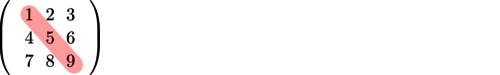
Figure 5.4: Illustration of the main diagonal of a matrix

Having named this as the main diagonal of a matrix then you can also define a diagonal matrix as one where the only place you might find non-zero elements is along the main diagonal.

It is clear that there are lots of possible diagonal matrices of a particular shape, because you can choose any numbers you wish to go along the main diagonal.

5.3.6 General pattern: Triangular matrices

These matrices are less important, and only used in more limited applications but we shall briefly mention them. There are actually two types of triangular matrices:

A matrix is called upper-triangular if the triangle of elements below the main diagonal are all zero; and
A matrix is called lower-triangular if the triangle of elements above the main diagonal are all zero.

This mismatch between “upper” and “below,” and between “lower” and “above” might sound like madness. However, it’s like our first definition of a diagonal matrix as one which is “zero in places not on the diagonal.” In fact there are two more natural and perfectly equivalent descriptions, namely

A matrix is called upper-triangular if only the triangle of elements including and above the main diagonal are allowed to be non-zero;
A matrix is called lower-triangular if only the triangle of elements including and below the main diagonal are allowed to be non-zero.

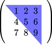
A picture of the upper-triangle highlighted, this matrix is not upper-triangular, because the entries below the triangle aren't all zeros.

Figure 5.5: A picture of the upper-triangle highlighted, this matrix is not upper-triangular, because the entries below the triangle aren’t all zeros.

The single word triangular is used to describe either or both of these cases above. Just like you can talk of African elephants and Indian elephants as special examples of elephants.

We shan’t dwell on this adjective for now, but just show a few examples of triangular matrices. First a few upper-triangular ones,

\[ \begin{pmatrix}1 & 4 \\ 0 & -3 \end{pmatrix}, \begin{pmatrix}0 & 2 \\ 0 & 1 \end{pmatrix}, \begin{pmatrix}2 & 0 & 8 \\ 0 & 1 & -2 \\ 0 & 0 & 3 \end{pmatrix}\]

then a few lower-triangular ones,

\[ \begin{pmatrix}1 & 0 \\ 4 & -3 \end{pmatrix}, \begin{pmatrix}1 & 0 \\ 3 & 0 \end{pmatrix}, \begin{pmatrix}2 & 0 & 0 \\ 3 & 1 & 0 \\ 4 & -1 & 2 \end{pmatrix}\]

finally a few that are not triangular at all,

\[ \begin{pmatrix}1 & 2 \\ 4 & -3 \end{pmatrix}, \begin{pmatrix}0 & 1 \\ 2 & 0 \end{pmatrix}, \begin{pmatrix}2 & -1 & 3 \\ 0 & 1 & 7 \\ 1 & 0 & 2 \end{pmatrix}\]

5.3.7 General pattern: Symmetric matrices

These types of matrices do arise a lot more in applications. They are also easy to identify just by looking at the entries of the matrix. The technical definition, which uses the word transpose from above, is to say that a matrix is symmetric if the transpose of the matrix is the same as the starting matrix.

The easier definition would be to say:

the matrix has a square shape, and
if you place a mirror down the main diagonal, then every number above the diagonal matches its image below the diagonal and vice-versa⁸⁵.

Here are some examples of symmetric matrices from which it will hopefully become obvious.

\[\begin{equation} \begin{pmatrix}5 & -1 & 2 \\ -1 & 3 & 4 \\ 2 & 4 & 0 \end{pmatrix}, \text{ and } \begin{pmatrix}1 & 0 & 8 & -4 \\ 0 & 3 & 7 & 11 \\ 8 & 7 & 2 & 9 \\ -4 & 11 & 9 & -2 \end{pmatrix} \end{equation}\]

Notice that along the main diagonal you can put whatever values you wish, but every other element has a mirror image element across the main diagonal.

In fact the matching mirror image location for the \((i,j)\)-element is the one in position \((j,i)\), e.g. Row 3 Column 1 must match Row 1 Column 3, and Row 2 Column 4 must match Row 4 Column 2.

5.3.8 Special quantity: The Determinant (important enough to have its own section below)

For every square matrix we can calculate a quantity known as the determinant. The process to calculate the determinant is easy for a \(2\)-by-\(2\) matrix but becomes progressively harder and messier for larger and larger matrices. We shall start with defining it for a \(2\)-by-\(2\) matrix.

For a \(2\)-by-\(2\) matrix which looks like this:

\[ \begin{pmatrix}a & b \\ c & d \end{pmatrix}\]

its determinant is defined to be the value of

\[ a\times d - b \times c \]

It’s just the product of the main diagonal, minus the product of the other diagonal.

Notationally, the determinant of a matrix called \(M\) is normally written \(\det(M)\).

Here is an image showing which pairs are multiplied, check the definition above to see which product is subtracted from the other product.

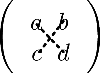
Figure 5.6: Illustration of products for finding a 2-by-2 deteminant.

Here are three example calculations, along with the \(\det\) notation illustrated:

\[ \det \begin{pmatrix}4 & 7 \\ 1 & 2 \end{pmatrix}= 4 \times 2 - 7 \times 1 = 1 \]

\[ \det \begin{pmatrix}-1 & 2 \\ -3 & -4 \end{pmatrix}= (-1) \times (-4) - 2 \times (-3) = 4+6=10 \]

\[ \det \begin{pmatrix}1 & 4 \\ -1 & -4 \end{pmatrix}= 1 \times (-4) - 4 \times (-1) = -4+4=0 \]

Take extreme care when calculating determinants when negative numbers are around. You will frequently be subtracting negative numbers, and need to convert two negatives into a plus.

Now for the \(3\)-by-\(3\) determinant…

Calculating the determinant always involves using every element of the matrix, so when we get to \(3\)-by-\(3\) it’s not the same pattern of diagonals. However, the formula for the \(3\)-by-\(3\) determinant can be described in terms of three \(2\)-by-\(2\) matrix determinants.⁸⁶

Let’s suppose we have a general \(3\)-by-\(3\) matrix that looks like this:

\[ \begin{pmatrix}a_{1,1} & a_{1,2} & a_{1,3} \\ a_{2,1} & a_{2,2} & a_{2,3} \\ a_{3,1} & a_{3,2} & a_{3,3} \end{pmatrix}\]

We have named each element by its location to make what follows easier to understand.

Definition of the \(3\)-by-\(3\) matrix determinant

One way to calculate the \(3\)-by-\(3\) determinant is to evaluate:

\[{\small a_{1,1} \times \det \begin{pmatrix}a_{2,2} & a_{2,3} \\ a_{3,2} & a_{3,3} \end{pmatrix}- a_{1,2}\times\det\begin{pmatrix}a_{2,1} & a_{2,3} \\ a_{3,1} & a_{3,3} \end{pmatrix}+ a_{1,3} \times \det\begin{pmatrix}a_{2,1} & a_{2,2} \\ a_{3,1} & a_{3,2} \end{pmatrix}} \]

This calculation is most easily understood via three pictures, or via watching the subsequent video showing it in action. Geometrically, the \(2\)-by-\(2\) determinants required are the ones you are left with if you delete Row 1 and sequentially Columns 1, 2 and 3 from the matrix like this:

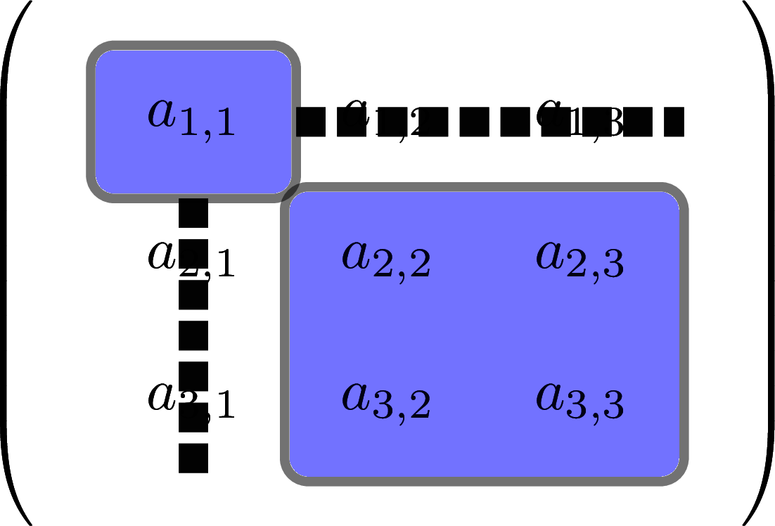
Figure 5.7: The lower square is the first 2-by-2 determinant needed to find a 3-by-3 determinant

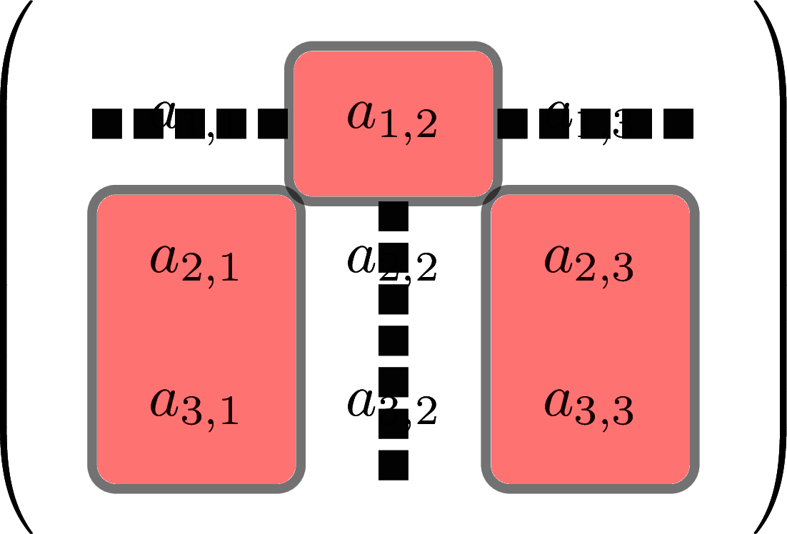
Figure 5.8: The lower split square is the second 2-by-2 determinant needed to find a 3-by-3 determinant

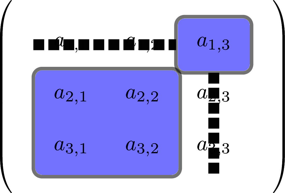
Figure 5.9: The lower square is the third 2-by-2 determinant needed to find a 3-by-3 determinant

Here is a video demonstration, which helps explain the procedure:

Alternative direct video link: https://gcu.planetestream.com/View.aspx?id=5354~4r~SDdzPCeX

In a direct link to the Vectors section, we can now present a formula for the Vector Product of two vectors using this \(3\)-by-\(3\) determinant.

You may recall Equation (4.9) provided a general formula for the Vector Product, namely

\[\begin{equation} \begin{pmatrix} a\\b\\c \end{pmatrix} \times \begin{pmatrix} d \\ e \\ f \end{pmatrix} = \begin{pmatrix} bf-ce \\ cd-af \\ ae-bd \end{pmatrix} \end{equation}\]

Well, another way to write this is:

\[\begin{equation} \begin{pmatrix}a\\b\\c \end{pmatrix}\times \begin{pmatrix}d \\ e \\ f \end{pmatrix}= \det \begin{pmatrix}\underline{i} & \underline{j} & \underline{k} \\ a & b & c \\ d & e & f \end{pmatrix} \tag{5.3} \end{equation}\]

where we recall that \(\underline{i},\underline{j},\underline{k}\) are just names for \(\begin{pmatrix}1\\0\\0\end{pmatrix}\), \(\begin{pmatrix}0\\1\\0\end{pmatrix}\) and \(\begin{pmatrix}0\\0\\1\end{pmatrix}\), respectively.

In words, we place our two given vectors into the second and third rows of a \(3\)-by-\(3\) matrix, and write the letters \(\underline{i},\underline{j},\underline{k}\) on the top row. Then we can calculate the determinant, giving the answer in terms of \(\underline{i}, \underline{j}\) and \(\underline{k}\). The answer will be the Vector Product of the vectors visible in Row 2 and Row 3.

It is important to put the vectors into the matrix in the same order they appeared in the Vector Product, otherwise your answer will be incorrect⁸⁷. The first vector in the Vector Product must go in Row 2, and the second vector in the Vector Product must go in Row 3.

Practice

Calculate the Vector Product of the two vectors from (4.10), namely \[ \underline{v}=\begin{pmatrix} 4\\1\\-5\end{pmatrix} \textrm{ and } \underline{w}=\begin{pmatrix} 2 \\ -9 \\ -3 \end{pmatrix} \] by using the determinant formula above.

Check your answer with the answer calculated in Section 4.13 after Equation (4.10).

Warning: this can get numerically messy, and easy to make mistakes.

5.3.9 Revision exercises

This section contained a large number of new words, adjectives, nouns and terminology. So it will be useful to try a few exercises to revise this topic before moving on.

Examples to try

For each of the following matrices determine if it is an example of any of our special matrices, or fits any of the general patterns. As a reminder here are the key terms we are using: (we won’t bother with triangular as it’s not that useful)

Square
Zero
Identity
Diagonal
Symmetric

\[ A = \begin{pmatrix}3 & 1 \\ 1 & 8 \end{pmatrix}\] \[ B = \begin{pmatrix}2 & 0 \\ 0 & 7 \end{pmatrix}\] \[ C = \begin{pmatrix}2 & 3 & 7 \\ 0 & 4 & 1 \end{pmatrix}\] \[ D = \begin{pmatrix}1 & 0 & 0 \\ 0 & 1 & 0 \\ 0 & 0 & 1 \end{pmatrix}\] \[ E = \begin{pmatrix}0 & 0 \\ 0 & 0 \end{pmatrix}\]

We shall, in fact, go through these examples quickly to ensure some of the special cases are ironed out upon first study.

Answers, explained:

Square: \(A\), \(B\), \(D\) and \(E\) are all square matrices. Their number of rows matches their number of columns.

Zero: Only \(E\) is an example of a zero matrix. Remember, every element must be zero, not just some of them.

Identity: Only \(D\) is an example of an identity matrix, in this case it is the \(3\)-by-\(3\) identity, often called \(I_3\).

Diagonal: \(B\) is a typical example of a diagonal matrix, all entries not on the main diagonal are zero. In fact \(D\) and \(E\) are technically also both diagonal – however observing they are an identity and zero matrix, respectively, provides even more information.

Symmetric: Here \(A\) is a typical example of a symmetric matrix. However, \(B\), \(D\) and \(E\) are all technically examples too because they are each identical to their own transpose.

Link to Numbas on the web

5.4 The inverse of a matrix

When we work in standard algebra we often deal with equations that look like \(8x = 3\), for which we divide both sides by \(8\) to reach \(x=\frac{3}{8}\). This division by \(8\) is the equivalent to multiplying both sides by \(8^{-1}\) because \(8 \times 8^{-1}=1\). However, when we’re working with matrices there is no easy way to define division by a matrix, but we can try. We shall only try and consider division/inversion by square matrices.

So if we have an equation like

\[ AB = C \]

where \(A\), \(B\) and \(C\) are matrices, and \(A\) is furthermore square-shaped, then there isn’t a guaranteed way to divide both sides by \(A\) to get \(B=\) something. The reason for this is that there isn’t always a single matrix \(B\) that works in that equation⁸⁸.

Let’s see an example. Suppose we have an equation like \(AB=C\) of the form: (here \(B\) is a \(2\)-by \(2\) matrix)

\[\begin{equation} \begin{pmatrix}1 & 2 \\ 2 & 4 \end{pmatrix}\Bigg(\;\;\: B \:\;\; \Bigg) = \begin{pmatrix}4 & 3 \\ 8 & 6 \end{pmatrix} \tag{5.4} \end{equation}\]

You would like to divide both sides by \(\begin{pmatrix}1 & 2 \\ 2 & 4 \end{pmatrix}\) to discover what \(B\) is. However, this isn’t possible because there are infinitely many matrices \(B\) that work! For example, \(B=\begin{pmatrix}2 & -1 \\ 1 & 2 \end{pmatrix}\) and \(B=\begin{pmatrix}0 & 1 \\ 2 & 1 \end{pmatrix}\) both work, and there are many more!

Sometimes it is possible, and there is a unique answer for \(B\). This process of trying to divide by \(A\) in an equation like \(AB=C\) to find \(B\) requires trying to find what is called the inverse of \(A\).

The inverse of a (square) matrix

Firstly, we only try and do this for square matrices.

We use the notation \(A^{-1}\) for what we call the inverse of matrix A.

By direct comparison with \(8^{-1}\) (the inverse of \(8\) being the number which multiplies \(8\) to give \(1\)), a matrix \(Z\) is called the inverse of matrix \(A\) if

\[ ZA = I \]

where \(I\) is an identity matrix. When such a matrix \(Z\) exists then we can write it as \(Z=A^{-1}\), and we say that \(A\) is invertible⁸⁹.

Warning: You cannot always find an inverse of a square matrix. Some square matrices don’t have inverses, while for non-square matrices none of this even makes sense. Mathematically, however, the good news is that most square matrices can be inverted. Whether an inverse exists depends on the determinant being non-zero.

Some examples of inverses:

If \(A=\begin{pmatrix}1 & 2 \\ 0 & 5 \end{pmatrix}\) then \(A\) does have an inverse and it is \[ A^{-1} = \begin{pmatrix}1 & -\frac{2}{5} \\ 0 & \frac{1}{5} \end{pmatrix}. \]

If \(A = \begin{pmatrix}4 & 1 \\ 5 & 2 \end{pmatrix}\) then \(A\) does have an inverse and it is \[ A^{-1} = \begin{pmatrix}\frac{2}{3} & -\frac{1}{3} \\ -\frac{5}{3} & \frac{4}{3} \end{pmatrix}. \]

You should check that in each of those examples, that

\[ A^{-1} A = \begin{pmatrix}1 & 0 \\ 0 & 1 \end{pmatrix}= I_2.\]

Note: it is also always true that \(AA^{-1}=I\) but we won’t discuss this here.

You will note that in both of the examples above the inverse of \(A\) contained fractions with the same denominator, which actually turns out to be the determinant of \(A\)! This is because there is a general formula for the inverse of a \(2\)-by-\(2\) matrix and it’s defined as follows:

Inverse of a \(2\)-by-\(2\) matrix formula

For any \(2\)-by-\(2\) matrix, \(A\), if the determinant of \(A\) isn’t zero (i.e. \(\det(A)\neq 0\)), then when

\[ A = \begin{pmatrix}a & b \\ c & d \end{pmatrix}\]

its inverse is

\[\begin{equation} A^{-1} = \frac{1}{\det(A)} \begin{pmatrix}d & -b \\ -c & a \end{pmatrix}, \tag{5.5} \end{equation}\] recalling that \(\det(A)=ad-bc\).

Warning: This formula doesn’t work if the determinant is zero.

In the case that \(ad-bc=0\) there is no inverse of \(A\).

Now go back to Equation (5.4) and check that the \(A\) matrix is not invertible⁹⁰.

It is worth taking a moment to look at the formula for the inverse of a \(2\)-by-\(2\) matrix in Equation (5.5).

Notice the pattern:

the main diagonal elements (the \(a\) and \(d\)) have been swapped;
the off-diagonal elements (the \(b\) and \(c\)) have had their signs changed⁹¹.

Then this result has been divided by the determinant.

Unfortunately this formula just needs to be memorized, and the general formula for the inverse of \(3\)-by-\(3\) matrices is much messier. The good news is that this quantity called the determinant can still be used as the deciding factor in all cases as to whether or not you can invert a matrix.

The determinant rule:

You can always find the inverse of a matrix if its determinant is not zero.
But if the determinant is zero, there is no inverse to find.

Why do we care about inverting a matrix?

Inverses will turn out to be really powerful. They can be used in a wide range of applications to solve equations involving matrices, because they allow us to perform simplifying algebra. Without them we are very limited in what we can do with algebra of matrices.

We shall consider the inverse of \(3\)-by-\(3\) and larger matrices in later sections (i.e. Sections 5.7 and 5.8).

First some examples to revise determinants, and inverses.

Practice

Below are four \(2\)-by-\(2\) matrices, in each case do the following:

Calculate its determinant;
Comment on whether the matrix will have an inverse;
If an inverse exists, find it!
After finding an inverse, multiply it by the original matrix to verify you get \(I_2\).

\[A = \begin{pmatrix}1 & 4 \\ 2 & 9 \end{pmatrix}\] \[B = \begin{pmatrix}-3 & -2 \\ 4 & 2 \end{pmatrix}\] \[C = \begin{pmatrix}2 & -8 \\ -1 & 4 \end{pmatrix}\] \[D = \begin{pmatrix}5 & 3 \\ 3 & 1 \end{pmatrix}\]

In more advanced courses on matrices you will see their applications. In the realm of 3D graphics and integration the determinant will turn out to have a geometric interpretation of how much the world is scaled when using a particular matrix. However we won’t go into that topic here.

5.5 Properties of inverse matrices

Before moving on to some applications, we shall first see a few properties of inverses that can prove useful when performing algebra. These rules could be learned, or looked up when necessary. They don’t need to be memorized, but you will learn them with practice. More important is to know there are some rules and when first working with matrices to go and check them.

Useful algebra rules for matrices

In all examples below \(A\) and \(B\) are general matrices, and \(k\) is a non-zero scalar (constant).

The inverse of an inverse equals the original matrix, i.e. \[ (A^{-1})^{-1} = A. \]
The inverse of the product of two matrices equals the product of their inverses but in reverse order! i.e. \[ (AB)^{-1} = B^{-1}A^{-1}. \]
The inverse of a matrix multiplied by a scalar equals the inverse of the matrix multiplied by the inverse of the scalar, i.e. \[ (kA)^{-1} = \frac{1}{k} A^{-1}, \text{ note }k \neq 0.\]
The inverse of the transpose of a matrix equals the transpose of the inverse of the matrix, i.e. \[ (A^T)^{-1} = (A^{-1})^T. \]

5.6 How to solve a \(2\)-by-\(2\) linear system using a matrix

Although we don’t see highly practical real-world examples here, we can at least see a clever use of matrices to solve simultaneous equations. In the example presented below we limit it to just solving two simultaneous equations but, as we shall see later, the method can be applied to as many simultaneous equations as you wish.

Firstly, we want to see how matrices are related to simultaneous equations.

Consider the following two simultaneous equations:

\[\begin{alignat*}{3} x & {}+{} & 2y & {}={} & -1 \\ 4x & {}-{} & 3y & {}={} & 18 \end{alignat*}\]

The clever use of matrices is to notice that there is a way to write this pair of equations as a single matrix equation.

How to re-write simultaneous equations in matrix format

Simultaneous equations can always be rewritten as a single matrix equation. For the example seen above it becomes,

\[\begin{equation*} \begin{pmatrix}1 & 2 \\ 4 & -3 \end{pmatrix}\begin{pmatrix}x \\ y \end{pmatrix}= \begin{pmatrix}-1 \\ 18 \end{pmatrix} \end{equation*}\]

Expand out this single equation carefully and see it matches!

Row 1 of the matrix multiplied by \(\begin{pmatrix}x \\ y \end{pmatrix}\) equalling \(-1\) yields the first simultaneous equation, and
Row 2 of the matrix multiplied by \(\begin{pmatrix}x \\ y \end{pmatrix}\) equalling \(18\) yields the second simultaneous equation.

To illustrate the general method, we can give a general formula.

General matrix method for solving simultaneous equations

Given a totally general pair of simultaneous equations:

\[\begin{alignat*}{3} ax & {}+{} & by & {}={} & g \\ cx & {}+{} & dy & {}={} & h \end{alignat*}\]

where \(a,b,c,d,g\) and \(h\) are scalars; we wish to solve these equations to find the values of \(x\) and \(y\) which make both equations simultaneously true.

We can write the equations as a single matrix equation as follows:

\[\begin{equation} \begin{pmatrix}a & b \\ c & d \end{pmatrix}\begin{pmatrix}x \\ y \end{pmatrix}= \begin{pmatrix}g \\ h \end{pmatrix} \tag{5.6} \end{equation}\]

If we now let \(M=\begin{pmatrix}a & b \\ c & d \end{pmatrix}\) then

if \(M^{-1}\) exists we can multiply (on the left) both sides of (5.6) by \(M^{-1}\) to obtain:

\[\begin{equation} M^{-1} \begin{pmatrix}a & b \\ c & d \end{pmatrix}\begin{pmatrix}x \\ y \end{pmatrix}= M^{-1} \begin{pmatrix}g \\ h \end{pmatrix} \tag{5.7} \end{equation}\]

however \(M=\begin{pmatrix}a & b \\ c & d \end{pmatrix}\), so

\[ M^{-1} \begin{pmatrix}a & b \\ c & d \end{pmatrix}= M^{-1}M = I_2 = \begin{pmatrix}1 & 0 \\ 0 & 1 \end{pmatrix}. \]

This means that Equation (5.7) turns into, \[\begin{equation} I_2 \begin{pmatrix}x \\ y \end{pmatrix}= M^{-1} \begin{pmatrix}g \\ h \end{pmatrix}. \tag{5.8} \end{equation}\]

We know that multiplying by \(I\) makes no difference, it’s like multiplying a scalar by \(1\) (see Section 5.3.3), so this equation becomes \[\begin{equation} \begin{pmatrix}x \\ y \end{pmatrix}= M^{-1} \begin{pmatrix}g \\ h \end{pmatrix} \tag{5.9} \end{equation}\] We now have an equation which tells us exactly what \(x\) and \(y\) are, which is our target!

Just before we see a worked example, a vital observation:

In all algebraic work, when solving equations with matrices, the key idea is almost always to

multiply both sides of the equation by the inverse of some matrix.

This multiplication by an inverse will convert one of the products into an identity, and simplify the algebra. We saw this above, when trying to find a formula for \(\begin{pmatrix}x \\ y \end{pmatrix}\) in (5.6), (5.7), (5.8) and (5.9). Notice how the left of the equation changed between (5.6) and (5.9), that was all the result of multiplication by the correct inverse matrix.

Example

We shall solve our starting problem: \[\begin{alignat*}{3} x & {}+{} & 2y & {}={} & -1 \\ 4x & {}-{} & 3y & {}={} & 18 \end{alignat*}\]

We begin by writing it as: \[\begin{equation} \begin{pmatrix}1 & 2 \\ 4 & -3 \end{pmatrix}\begin{pmatrix}x \\ y \end{pmatrix}= \begin{pmatrix}-1 \\ 18 \end{pmatrix} \tag{5.10} \end{equation}\]

Next we let \(M = \begin{pmatrix}1 & 2 \\ 4 & -3 \end{pmatrix}\) and desire to find \(M^{-1}\).

First we calculate \(\det(M)=1\times (-3) - 2 \times 4 = -11\).

Second we use the general formula, from Equation (5.5)⁹²,

\[ M^{-1} = -\frac{1}{11}\begin{pmatrix}-3 & -2 \\ -4 & 1 \end{pmatrix}\]

Third we perform our key step: we multiply (on the left) both sides by \(M^{-1}\) with the intention of cancelling out the existing \(M\) on the left.

So we multiply Equation (5.10) by \(M^{-1}\) to get

\[\begin{equation} M^{-1} \begin{pmatrix}1 & 2 \\ 4 & -3 \end{pmatrix}\begin{pmatrix}x \\ y \end{pmatrix}= M^{-1} \begin{pmatrix}-1 \\ 18 \end{pmatrix} \tag{5.11} \end{equation}\]

To see the algebra in gory detail we substitute our value of \(M^{-1}\).

The left side looks like:

\[\begin{equation*} \text{Left}=-\frac{1}{11}\begin{pmatrix}-3 & -2 \\ -4 & 1 \end{pmatrix}\begin{pmatrix}1 & 2 \\ 4 & -3 \end{pmatrix}\begin{pmatrix}x \\ y \end{pmatrix} \end{equation*}\]

and the right side looks like:

\[\begin{equation*} \text{Right}=-\frac{1}{11}\begin{pmatrix}-3 & -2 \\ -4 & 1 \end{pmatrix}\begin{pmatrix}-1 \\ 18 \end{pmatrix} \end{equation*}\]

and these two sides are equal.

However, \(-\dfrac{1}{11}\begin{pmatrix}-3 & -2 \\ -4 & 1 \end{pmatrix}\begin{pmatrix}1 & 2 \\ 4 & -3 \end{pmatrix}= \begin{pmatrix}1 & 0 \\ 0 & 1 \end{pmatrix}\), so Equation (5.11) becomes

\[\begin{equation*} I_2 \begin{pmatrix}x \\ y \end{pmatrix}= -\frac{1}{11}\begin{pmatrix}-3 & -2 \\ -4 & 1 \end{pmatrix}\begin{pmatrix}-1 \\ 18 \end{pmatrix}, \end{equation*}\]

and \(I_2 \begin{pmatrix}x \\ y \end{pmatrix}= \begin{pmatrix}x \\ y \end{pmatrix}\), so we reach:

\[\begin{equation*} \begin{pmatrix}x \\ y \end{pmatrix}= -\frac{1}{11}\begin{pmatrix}-3 & -2 \\ -4 & 1 \end{pmatrix}\begin{pmatrix}-1 \\ 18 \end{pmatrix}. \end{equation*}\]

These steps are the same every time we use this method⁹³. The answer to our problem now results from performing the multiplication on the right.

You should check by hand that you agree with

\[ -\frac{1}{11}\begin{pmatrix}-3 & -2 \\ -4 & 1 \end{pmatrix}\begin{pmatrix}-1 \\ 18 \end{pmatrix}= -\frac{1}{11}\begin{pmatrix}-33 \\ 22 \end{pmatrix}. \]

So,

\[\begin{equation*} \begin{pmatrix}x \\ y \end{pmatrix}= \begin{pmatrix}3 \\ -2 \end{pmatrix}, \end{equation*}\] and so \(x=3\) and \(y=-2\).

This calculation might look like a lot of work, but it is actually the same fundamental algebra every time, except that the matrices \(M\) and \(M^{-1}\), and the right-hand side will depend upon the problem being tackled. Here is the general shortcut answer…

Given simultaneous equations in the format:

\[ M\underline{x} = \underline{b}\] where

\(M\) is a square matrix;
\(\underline{b}\) is a column vector containing the right-hand side values; and
\(\underline{x}\) is a column vector containing the unknown variables, e.g. \((x,y)\), for which we wish to solve.

Then if \(M^{-1}\) exists⁹⁴ the answer is always \[\begin{equation*} \underline{x} = M^{-1} \underline{b}. \tag{5.12} \end{equation*}\]

Practice

In each of the following problems convert the simultaneous equations into a matrix equation, then use the above “matrix inverse method” to solve to find \(x\) and \(y\).

Note: It is easy to check your own answers, just substitute your solutions for \(x\) and \(y\) back into the original equations and confirm that they satisfy both equations.

Problem 1: Solve \[\begin{alignat*}{3} 4x & {}+{} & 2y & {}={} & 10 \\ 3x & {}-{} & 7y & {}={} & -1 \end{alignat*}\]
Problem 2: Solve \[\begin{alignat*}{3} 3x & {}-{} & 5y & {}={} & 17 \\ -x & {}-{} & 6y & {}={} & 2 \end{alignat*}\]

Warning:

In the case that the determinant of the \(2\)-by-\(2\) matrix is zero, then the matrix doesn’t have an inverse. Therefore we do not have a matrix to multiply both sides of the equations by, as in Equation (5.7), to convert the left hand side into \(I_2\begin{pmatrix}x \\ y \end{pmatrix}\).

Typically there will be infinitely many possible \((x,y)\) solutions to the equations. In very exceptional circumstances, however, there may be no solutions at all. We shall not go into these details here.

5.7 \(3\)-by-\(3\) matrices

There is fundamentally nothing particularly different to working with \(3\)-by-\(3\) matrices than with \(2\)-by-\(2\) matrices. All the adjectives discussed in Section 5.3 were intentionally designed to work for matrices of all sizes⁹⁵.

Using \(3\)-by-\(3\) matrices allows you to model three-dimensional situations, so in one sense you may expect them to be more useful for real-world modelling. However, we very often find in Engineering applications that we are working on cross-sectional areas, or by symmetry we are able to neglect one dimension – so a great deal of applications you will see actually only require working in two-dimensions.

One key difference, however, is the application of matrices for solving simultaneous equations, where the dimensions of the square matrix correspond to the number of equations. Thus we need \(3\)-by-\(3\) matrices to be able to solve sets of \(3\) simultaneous equations, and indeed \(n\)-by-\(n\) matrices to solve \(n\) simultaneous equations (see Section 5.8 later).

The only real differences mathematically are that:

the number of raw calculations required when multiplying \(3\)-by-\(3\) matrices is markedly increased;
the formula for the determinant is more complicated; and
there isn’t a nice easy formula for the inverse of a \(3\)-by-\(3\) matrix, like there was for a \(2\)-by-\(2\) matrix in (5.5).

We actually already gave a formula, and procedure for the determinant of the \(3\)-by-\(3\) matrix in Section 5.3.8, where you will have seen it’s considerably messier to calculate than finding a \(2\)-by-\(2\) determinant. However, whether a matrix has an inverse or not is still just a matter of whether its determinant is not zero or is zero.

There are a few different, equally good methods, for finding the inverse of a \(3\)-by-\(3\) matrix. In practice, the manual skill of finding such inverses is becoming less and less important in mathematics since software to find the inverse for you is readily available. As such these notes will not contain an explanation of the method. You are free to look up any good methods, these two are particularly popular and not too complicated:

Co-factor and adjoint method for matrix inverses,
Augmented matrix method for matrix inverses (also called the Gauss-Jordan method),

We shall discuss general computer methods briefly in the final Section 5.8.

For now, we shall just assume that we have a method for finding the inverse of a \(3\)-by-\(3\) matrix. The important fact you must know is that the inverse of a \(3\)-by-\(3\) matrix is a matrix which multiplied by the original matrix yields \(I_3\), the \(3\)-by-\(3\) identity matrix, e.g. \[\begin{equation*} \begin{pmatrix}1 & 4 & 0 \\ 2 & -1 & 7 \\ 1 & 8 & 9 \end{pmatrix}^{-1}\begin{pmatrix}1 & 4 & 0 \\ 2 & -1 & 7 \\ 1 & 8 & 9 \end{pmatrix}= \begin{pmatrix}1&0&0 \\ 0&1&0 \\ 0&0&1 \end{pmatrix} \end{equation*}\]

Let us use a matrix inverse to solve a system of three simultaneous equations.

Solve these simultaneous equations using the inverse matrix method:

\[\begin{alignat*}{4} 3x & {}+{} & y & {}+{} & z & {}={} & 1 \\ x & {}-{} & 2y & {}-{} & z & {}={} & 0 \\ 8x & {}-{} & 2y & {}+{} & z & {}={} & -3 \end{alignat*}\]

Assuming you already know that:

\[\begin{equation*} \begin{pmatrix} 3 & 1 & 1 \\ 1 & -2 & -1\\ 8 & -2 & 1 \end{pmatrix}^{-1} = \frac{1}{7}\begin{pmatrix}4 & 3 & -1 \\ 9 & 5 & -4 \\ -14 & -14 & 7 \end{pmatrix}. \end{equation*}\]

The first step is to convert our simultaneous equations into a single matrix equation. The three equations will become a single \(3\)-by-\(3\) matrix multiplied by a \(3\)-by-\(1\) column matrix, equal to another \(3\)-by-\(1\) column matrix, like this: \[\begin{equation*} \begin{pmatrix} 3 & 1 & 1 \\ 1 & -2 & -1\\ 8 & -2 & 1 \end{pmatrix}\begin{pmatrix}x\\y\\z \end{pmatrix}= \begin{pmatrix}1 \\0 \\-3 \end{pmatrix}. \end{equation*}\]

The next step is to find the inverse of our \(3\)-by-\(3\) matrix, which has already been done for us.

We then multiply both sides (on their lefts) by this inverse. So the left-hand side of the equation becomes: \[\begin{equation*} \frac{1}{7}\begin{pmatrix}4 & 3 & -1 \\ 9 & 5 & -4 \\ -14 & -14 & 7 \end{pmatrix} \begin{pmatrix} 3 & 1 & 1 \\ 1 & -2 & -1\\ 8 & -2 & 1 \end{pmatrix}\begin{pmatrix}x\\y\\z \end{pmatrix}, \end{equation*}\] and the right-hand side becomes \[\begin{equation*} \frac{1}{7}\begin{pmatrix}4 & 3 & -1 \\ 9 & 5 & -4 \\ -14 & -14 & 7 \end{pmatrix}\begin{pmatrix}1 \\0 \\-3 \end{pmatrix}, \end{equation*}\] putting them together and simplifying we get…

\[\begin{equation*} I_3 \begin{pmatrix}x\\y\\z \end{pmatrix}= \begin{pmatrix}x\\y\\z \end{pmatrix}= \frac{1}{7}\begin{pmatrix}4 & 3 & -1 \\ 9 & 5 & -4 \\ -14 & -14 & 7 \end{pmatrix}\begin{pmatrix}1 \\0 \\-3 \end{pmatrix}, \end{equation*}\] and it just remains to perform the matrix multiplication on the right hand side…

\[\begin{equation*} \frac{1}{7}\begin{pmatrix}4 & 3 & -1 \\ 9 & 5 & -4 \\ -14 & -14 & 7 \end{pmatrix}\begin{pmatrix}1 \\0 \\-3 \end{pmatrix}= \begin{pmatrix}1 \\ 3 \\ -5 \end{pmatrix}. \end{equation*}\] So \(x=1\), \(y=3\) and \(z=-5\).

Here is an example for you to try at home. Notice that you can just use the general result from Equation (5.12) once you have identified the necessary matrices in the question.

Practice

Solve these simultaneous equations using the inverse matrix method:

\[\begin{alignat*}{4} 4x & {}+{} & y & {}+{} & z & {}={} & 1 \\ x & {}-{} & 2y & {}-{} & z & {}={} & 0 \\ 8x & {}-{} & y & {}+{} & z & {}={} & -3 \end{alignat*}\]

You should look online for a \(3\)-by-\(3\) matrix inverse calculator, to find the necessary inverse. As an exercise check that the supplied inverse is correct by multiplying the original matrix by its inverse to (hopefully) obtain the identity matrix \(I_3\).

You can find many examples online if you wish to test your skills with this type of question, you will also find a couple of examples in the bonus exercises in Section 8.

5.8 Larger matrices

Larger matrices’ main use is for representing large numbers of simultaneous equations in one single equation. To represent \(n\) simultaneous linear equations in the matrix format will involve designing an appropriate \(n\)-by-\(n\) matrix. Useful applications normally require calculating this matrix’s inverse at some point.

Fortunately there are many efficient algorithms designed for computers to calculate inverses of large matrices. For humans it becomes extremely time consuming to calculate the inverse of matrices as they get larger, indeed humans will very rarely attempt to invert any matrix by hand which is larger than \(3\)-by-\(3\).

The only frequent exception to the previous claim about human calculation, is for certain special matrices whose inverses are actually easy to calculate. One interesting class of matrices like this are diagonal matrices (see Section 5.3.5). Recall that a diagonal matrix looks like this:

\[\begin{equation*} \begin{pmatrix} d_1 & 0 & 0 & 0 & \ldots &0 \\ 0 & d_2 & 0 & 0 & \ldots &0\\ 0 & 0 & d_3 & 0 & \ldots &0\\ 0 & 0 & 0 & d_4 & \ldots &0\\ \vdots & \vdots & \vdots & \vdots & \ddots &0\\ 0&0&0&0&0& d_n \end{pmatrix} \end{equation*}\]

All entries not on the main diagonal are zeros, and the diagonal entries can take any values you like.

Note: when working with large matrices we often use a sequence of three dots to say “continue the pattern.”

A typical \(4\)-by-\(4\) example may look like this:

\[\begin{equation*} \begin{pmatrix} 7 & 0 & 0 & 0 \\ 0 & -2 & 0 & 0 \\ 0 & 0 & \frac{1}{3} & 0 \\ 0 & 0 & 0 & 10 \end{pmatrix} \end{equation*}\]

Notice that finding the inverse is actually very easy. Just perform the following multiplication to see why,

\[\begin{equation*} \begin{pmatrix} \frac{1}{7} & 0 & 0 & 0 \\ 0 & -\frac{1}{2} & 0 & 0 \\ 0 & 0 & 3 & 0 \\ 0 & 0 & 0 & \frac{1}{10} \end{pmatrix} \begin{pmatrix} 7 & 0 & 0 & 0 \\ 0 & -2 & 0 & 0 \\ 0 & 0 & \frac{1}{3} & 0 \\ 0 & 0 & 0 & 10 \end{pmatrix}, \end{equation*}\]

the answer is just \(I_4\), notice how all the zeros make the product quite easy to calculate.

So inverting an \(n\)-by-\(n\) diagonal matrix really is just as simple as going down the diagonal and inverting each element one at a time, i.e. replacing \(d\) with \(d^{-1}\) or \(\frac{1}{d}\), however you prefer to write it. Just beware, this doesn’t work if any elements on the diagonal are zeros!

As discussed earlier, the primary use of larger matrices is for solving systems of simultaneous equations, though they can be more complicated than standard linear equations. These methods can be used, for example, to solve systems of what are called differential equations (which you will study in later courses).

A general set of \(n\) simultaneous linear equations looks like this: \[\begin{alignat*}{6} a_{1,1}x_1 & {}+{} & a_{1,2}x_2 & {}+{} & a_{1,3}x_3 & {}+{} & \ldots {}+{} & a_{1,n}x_n & {}={} & b_1 \\ a_{2,1}x_1 & {}+{} & a_{2,2}x_2 & {}+{} & a_{2,3}x_3 & {}+{} & \ldots {}+{} & a_{2,n}x_n & {}={} & b_2 \\ a_{3,1}x_1 & {}+{} & a_{3,2}x_2 & {}+{} & a_{3,3}x_3 & {}+{} & \ldots {}+{} & a_{3,n}x_n & {}={} & b_3 \\ \vdots\phantom{xyz} & {}{} & \vdots\phantom{xyz} & {}{} & \vdots\phantom{xyz} & {}{} & {}{} & \vdots\phantom{xyz} & {}={} & \vdots \\ a_{n,1}x_1 & {}+{} & a_{n,2}x_2 & {}+{} & a_{n,3}x_3 & {}+{} & \ldots {}+{} & a_{n,n}x_n & {}={} & b_n \end{alignat*}\] where all the \(a_{ij}\) and \(b_k\) are constants. And we had to name our variables \(x_1\), \(x_2\), \(x_3\) etc… else we would have quickly run out of letters!

Such a system of equations can always be written in matrix format as:

\[\begin{equation} A\underline{x} = \underline{b} \tag{5.13} \end{equation}\] where \[\begin{equation*} \underline{x} = \begin{pmatrix}x_1 \\ x_2 \\ x_3 \\ \vdots \\ x_n \end{pmatrix},\quad \underline{b} = \begin{pmatrix}b_1 \\ b_2 \\ b_3 \\ \vdots \\ b_n \end{pmatrix} \end{equation*}\] and \[\begin{equation*} A = \begin{pmatrix} a_{11} & a_{12} & a_{13} & \ldots & a_{1n} \\ a_{21} & a_{22} & a_{23} & \ldots & a_{2n} \\ a_{31} & a_{32} & a_{33} & \ldots & a_{3n} \\ \vdots & \vdots & \vdots & \ddots & \vdots \\ a_{n1} & a_{n2} & a_{n3} & \ldots & a_{nn} \end{pmatrix} \end{equation*}\]

The solution to Equation (5.13), assuming that \(det(A)\neq 0\), so that \(A\) has an inverse⁹⁶, is always \[\begin{equation*} \underline{x} = A^{-1}\underline{b} \tag{5.14} \end{equation*}\] The algebra to get from (5.13) to (5.14) has been seen twice before, first in Equations (5.7), (5.8), (5.9) for \(2\)-by-\(2\) matrices, and then again in (5.11) and (5.12) when working with \(3\)-by-\(3\) matrices. It always just involves multiplying on the left by the inverse of our square matrix, and simplifying.

Having glossed over the procedures for finding the inverse of a \(3\)-by-\(3\) matrix⁹⁷ we should conclude with some references to software you can use to find matrix inverses larger than \(2\)-by-\(2\) when needed.

Software for finding matrix inverses

online you will find various websites called things like matrix inverse calculator;
if using common spreadsheet software⁹⁸, there’s a function called MINVERSE (matrix inverse);
if using Wolfram Alpha you can type inv, inverse or inverse of;
in Python one option is numpy.linalg.inv();
in R, you can use inv or solve;
in Matlab you can use inv; and
in other software, just search the web or the help files.

Practice

Use one of the software options above to find the inverse of this \(4\)-by-\(4\) matrix: \[\begin{equation*} \begin{pmatrix} 3 & 1 & 0 & 5 \\ 0 & 1 & -1 & 2 \\ 2 & 5 & -2 & 4 \\ 1 & 0 & -1 & 3 \end{pmatrix} \end{equation*}\]

Verify your answer is the inverse by multiplying it by the matrix and verifying you get an identity matrix.

5.9 Summary of chapter

Having worked through this chapter and attempted the exercises you should now have developed understanding of the following topics:

Know what a matrix is and describe its shape;
Perform basic algebra including addition, subtraction and scalar multiplication;
Determine if matrices are valid shapes to be multiplied together, and carry out the multiplication where appropriate;
Calculate the determinant of \(2\)-by-\(2\) and \(3\)-by-\(3\) matrices;
Calculate the inverse of \(2\)-by-\(2\) matrices, when it exists; and
Use matrix methods to solve systems of linear equations.

4 Vectors

6 Algebra exercises