4 Vectors

Vectors are useful mathematical objects for describing, simultaneously, a real-world quantity with length and accompanying direction. For travel purposes, a vector might describe moving North for 3 kilometres – the direction being North, and the length³⁷ being 3 kilometres. This scenario is an example of what is called a displacement vector: a vector which describes a physical displacement (a ‘movement’). Vectors can also describe other real-world phenomena, especially in the area of mechanics, such as forces, velocity and even momentum. A proper description of a force involves the size or strength³⁸ of the force, together with a direction in which the force is acting. For example, when studying a mechanics problem with gravity the force of gravity will have a strength (in Newtons) and a direction (downwards).

Given their description, vectors can always be described geometrically by a line segment with an arrowhead. The length of the segment describes the length of the vector, and the way the line points (with the arrowhead) gives the direction. Here are some 2-dimensional examples, in Figure 4.1:

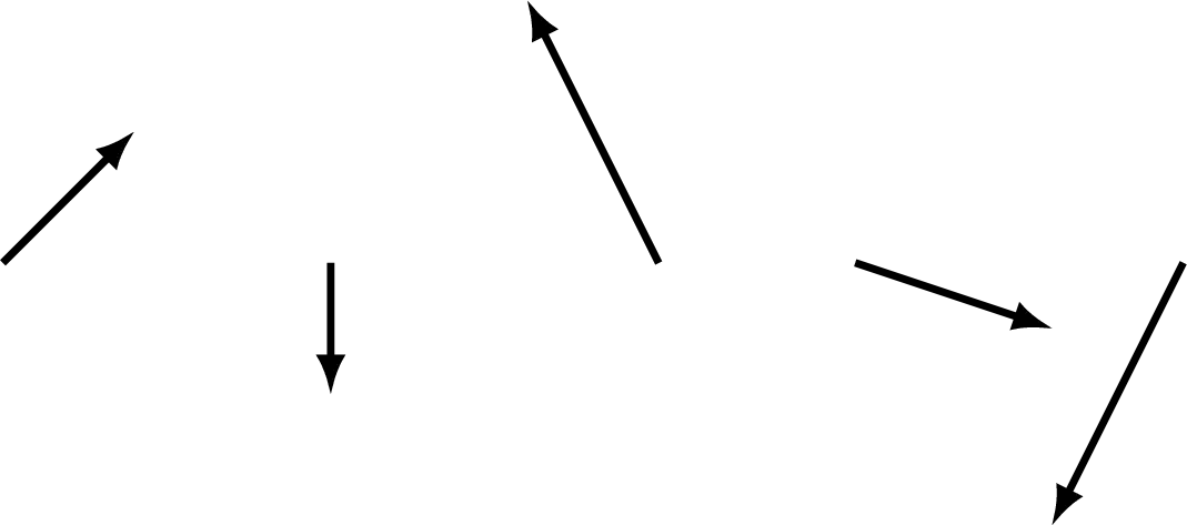
Figure 4.1: Some examples of vectors

Where a vector is drawn is not important, only its length and direction, so two vectors can be identical and just drawn in different locations. In Figure 4.2 are five vectors, they are all the same vector, just drawn in different places:

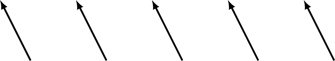
Figure 4.2: Five identical vectors

4.1 Scalars and vectors

Vectors differ from what are called scalars in one specific way, a scalar is just single number used to describe a length/size/strength/magnitude³⁹ and doesn’t include a direction. Scalars are therefore nothing special at all, and just another name for any quantified physical quantity, like temperature, voltage, distance, height, mass, volume, density and many many more. All of these quantities are describable with a single value (and accompanying units) such as a voltage of 9 volts, a temperature of \(21.4^{\circ}\)C, a density of \(450\) kg m^-3, or mass of \(74\) kg. When performing algebra and calculations we often neglect the units (re-inserting them at the end) and so a scalar is just a number like \(9\) or \(21.4\).

Vectors, on the other hand additionally always include a direction, such as the example ‘\(3\)km North’ earlier, a velocity like ‘\(45\)ms^-1 East,’ or ‘a force of \(10\)N acting at an angle \(30\) degrees anticlockwise from the horizontal.’

Beware: when talking about vectors there a few quantities that have specific mathematical meanings, which can differ from how they are sometimes used in common English language.

The first common example concerns speed and velocity:

• Speed – this is a scalar and refers purely to how fast something is travelling.
• Velocity – this is a vector and tells you both speed and direction.

So it is mathematically wrong to say someone has velocity of \(20\) miles per hour, that is their speed.

The second common example concerns distance and displacement:

• Distance – this is a scalar and refers purely to how far apart two places are.
• Displacement – this is a vector and refers to the movement required between two places, so includes a distance and direction.

So it is mathematically wrong to say an object has experienced a displacement of \(10\) metres. You need to also specify in what direction it moved if you want to call it a displacement. Alternatively it would be fine to just say it has moved a distance of \(10\) metres, but this is less descriptive.

4.2 Notation for vectors

4.2.1 Fonts for vectors

Mathematically it’s very tedious, not very productive, and pretty imprecise to have to refer to directions of vectors in terms of compass points like we have done above. It makes a lot more sense to agree some good notation instead.

We begin with the first good notation. If we are talking about a vector and want to give it an algebraic name like \(v\) (note this is the English letter v in italic maths font⁴⁰) then we underline the letter, so we in fact write \(\underline{v}\) which signifies that it represents a vector not a scalar.

This approach can make it easier to read equations which contain vectors and scalars. The bad news for students is that it’s not universally agreed as a notation, and some authors just use bold, and so write \(\bf{v}\) instead. Yet more authors instead place a tiny arrow on top of the letter, and write \(\vec{v}\).

For consistency we shall try and use just the underline notation in these notes, so we’ll write \(\underline{a}\), \(\underline{b}\), \(\underline{u}\), \(\underline{v}\) etc…

4.2.2 Mathematical representation

The more interesting question is how to actually describe the length and direction in a clean, and easy way. The answer is that a number of good methods have been invented, and the best way generally depends upon the context of what you wish to do with your vector. Consequently there are a few totally equivalent but different-looking ways to represent a vector. We shall discuss the different representations or formats in later sections.

For now we just introduce them by name:

• Polar format – here you describe the length and then the direction (as an angle from the horizontal).
• Rectangular/Cartesian format – here you use the good old standard \((x,y)\) axes as your basis.
• Geometric format – here you draw an arrow of a particular length (not very useful except in hand-drawings).

In addition, inside the rectangular format we shall see there is a very convenient bracket notation used too, sometimes called matrix format.

4.3 Cartesian/Rectangular notation

We begin with probably the easiest to understand notation. We start with a vector like this one, which has length \(\sqrt{13}\approx 3.606\) and makes an angle of \(33.69\) degrees, measured in the anticlockwise direction, with the horizontal (see Figure 4.3):

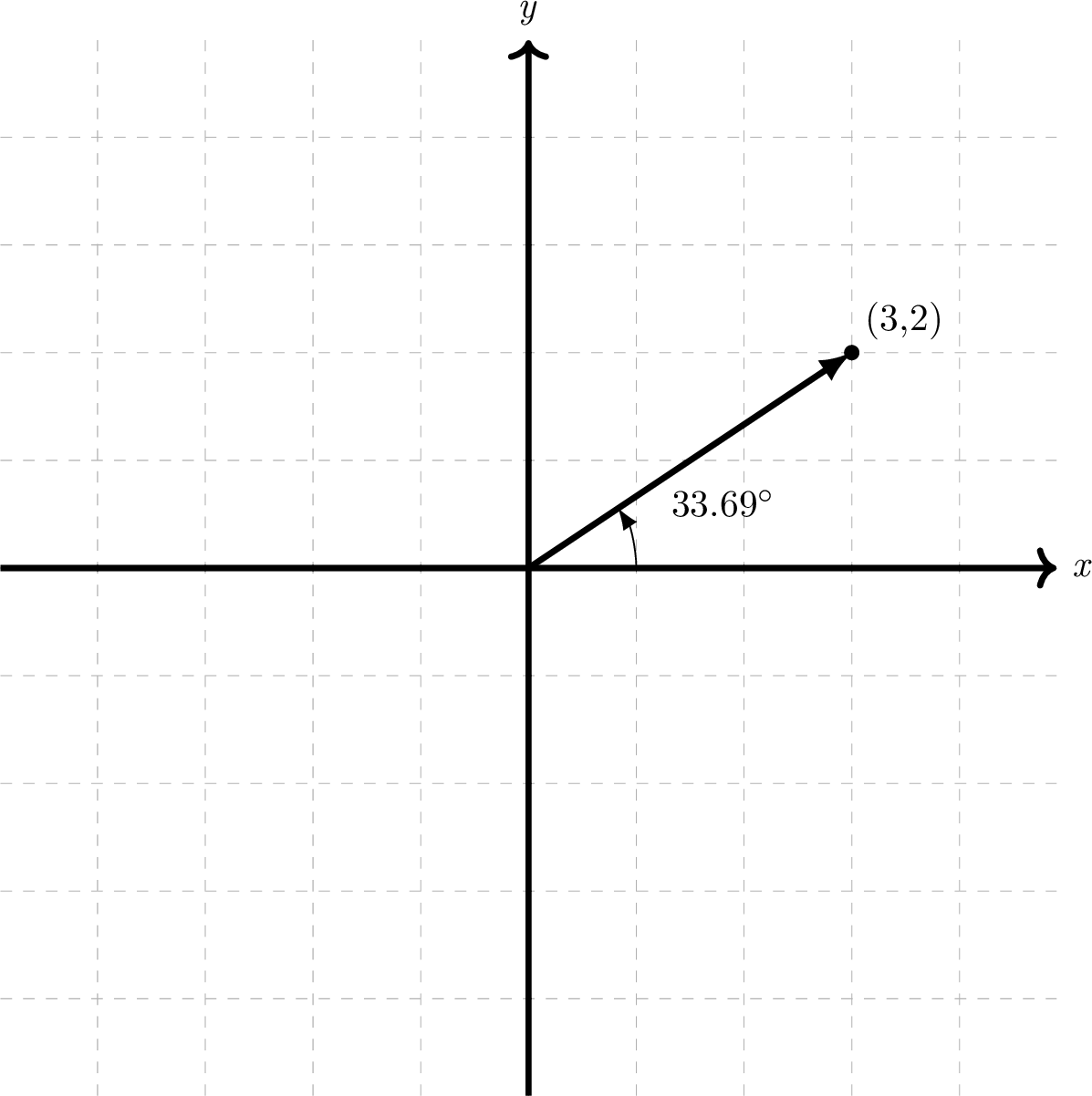
Figure 4.3: A vector of length \(\sqrt{13}\approx 3.606\) at an angle of \(33.69^{\circ}\).

The choice of \(\sqrt{13}\) was special so that our vector represents a horizontal movement of \(+3\) and vertical movement of \(+2\). It is very typical for the length to be a surd⁴¹, in fact it is to be expected if the horizontal and vertical lengths are both integers. You can use trigonometry (SOH-CAH-TOA) to check that \(\tan(33.69^{\circ})=\frac{2}{3}\)⁴².

This vector can be described, rather than by the length and direction, by its horizontal and vertical movements. Note that it didn’t need to be drawn starting at the origin, but it just made it easier to see the movements. The way we write this vector in rectangular format is as \((3,2)\).

Rectangular (also called Cartesian⁴³) format for a vector involves working out the horizontal and vertical movement represented by the vector’s arrow. Then placing them in a bracket of format

\[ (x,y) \]

where the first component, \(x\), represents the horizontal movement, and the second component, \(y\), represents the vertical component.

How to remember which way around to write the components?

A common way to remember which component is which is via this alphabet-based memory aid…

fiRst = Rows

seCond = Columns

Where Rows refers to horizontal movements, and Columns refers to vertical movements.

Let’s see a worked example:

Identify in the picture below the following five vectors: \((1,2),(-3,-1),(2,1),(-1,3),(-3,0)\) you may assume the dotted grid lines are spaced \(1\) unit apart.

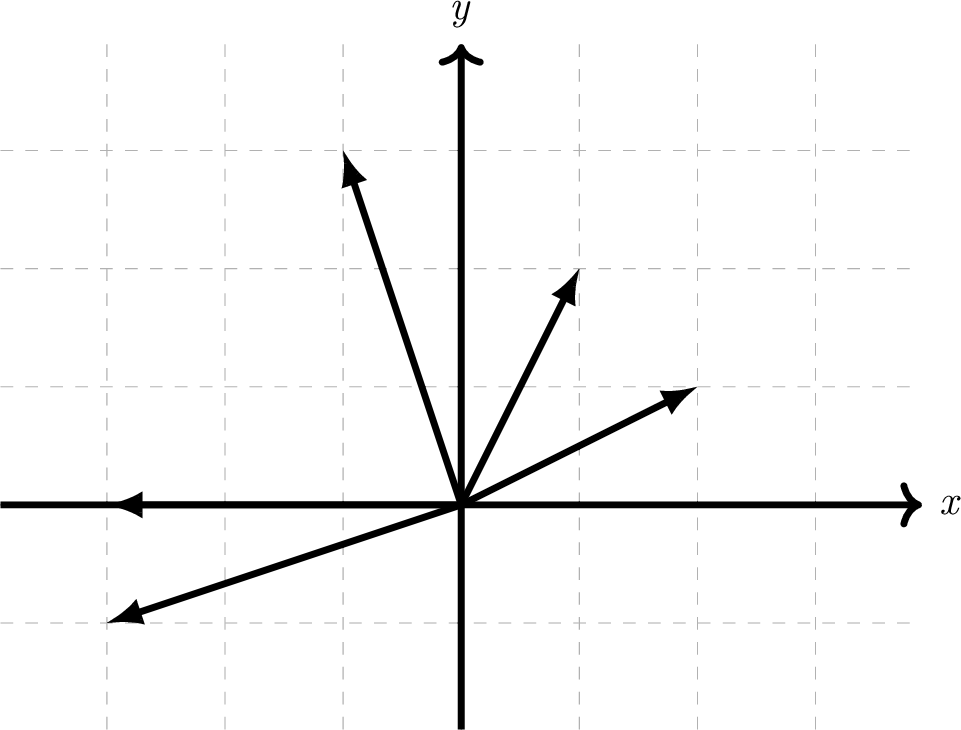
Figure 4.4: Five vectors for you to label using their rectangular format

The answers have been labelled on the picture below:

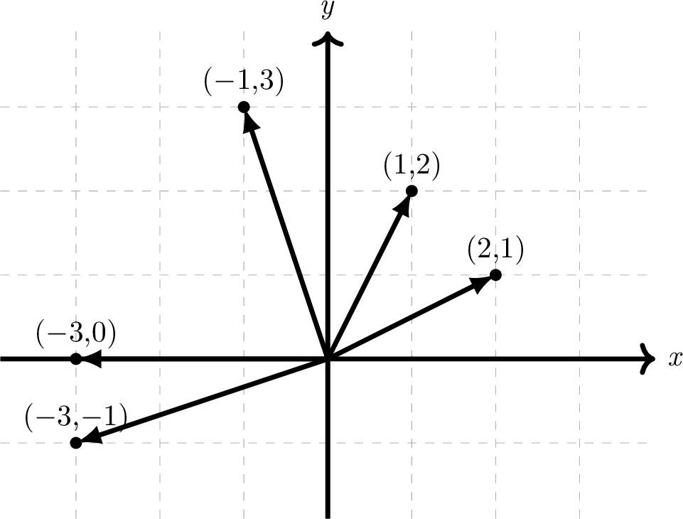
Figure 4.5: Five vectors labelled in rectangular format

There is sometimes confusion between this vector format and the \(x,y\) notation you’ve used in the past to identify points on a graph (remember the vector is really the line joining the origin to this point). For this reason, many people prefer to use what is called the matrix or column vector format which merely involves writing the vector vertically rather than horizontally on the page. Matrix (and it’s plural matrices) is a specific mathematical term for a grid of numbers inside brackets – matrices are covered in separate chapter.

Here are the five vectors, \((2,1),(1,2),(-1,3),(-3,-1),(-3,0)\), from our example above written in matrix format:

\[ \begin{pmatrix} 2 \\ 1 \end{pmatrix}, \begin{pmatrix} 1 \\ 2 \end{pmatrix}, \begin{pmatrix} -1 \\ 3 \end{pmatrix}, \begin{pmatrix} -3 \\ -1 \end{pmatrix}, \begin{pmatrix} -3 \\ 0 \end{pmatrix}. \]

This format takes up more space in writing, but does have the benefit of being obviously a vector rather than describing a point. We shall later see that there is another format to write rectangular notation by introducing some base vectors called \(\underline{i}\) and \(\underline{j}\), but we won’t use them yet.

4.4 Polar notation

Polar notation is perhaps the easiest notation to understand, but unfortunately isn’t very useful in a lot of algebra applications. This notation fits nicely with our original geometric introduction of vectors, here is a summary.

The polar format of a vector involves drawing the vector starting at the origin on a graph and describing two quantities:

• the length of the vector
• the angle the vector makes anticlockwise with the positive \(x\)-axis

The length is normally called \(r\), and is always chosen to be positive⁴⁴.

The angle is normally called \(\theta\) (the Greek letter theta) and we shall choose to describe it as between \(-180^{\circ}\) and \(+180^{\circ}\). This means we don’t write \(200^{\circ}\) but we write \(-160^{\circ}\) instead⁴⁵. This range of values is really just another notational choice, so you’ll find some authors use the range of \(0^{\circ}\) to \(+360^{\circ}\) for \(\theta\). Such authors will use \(200^{\circ}\) rather than \(-160^{\circ}\).

The notation itself is written either as \((r,\theta)\) or \(r \angle \theta\), with the former being more popular. You do need to remember that the first number is always the length and the second number the angle. However, if you include the degree symbol, \({}^{\circ}\), it will be obvious.

Figure 4.6 is the same basic example seen in the introduction of the rectangular notation:

Figure 4.6: A vector of length \(\sqrt{13}\approx 3.606\) at an angle of \(33.69^{\circ}\).

This vector is easy to describe in polar notation as \((r,\theta)=(\sqrt{13},33.69^{\circ})\)

Figure 4.7 shows three more vectors that can be described via their length and angle.

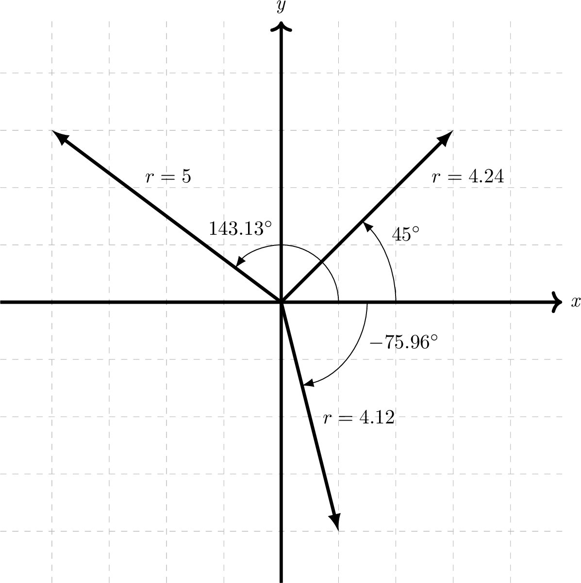
Figure 4.7: Three vectors with their angles and lengths labelled.

Notice the angle of the vector is always measured starting from the positive \(x\)-axis (this is called the pole, as in polar).

Notice also that the vector which points downwards has a negative angle, because we measure anticlockwise angles as positive, and clockwise as negative, with the positive positive \(x\)-axis measured as zero.

Here is a practice example:

Identify in the picture below the following three vectors written in polar notation: \((1.41,45^{\circ}),(5,126.87^{\circ}),(3.61,-123.69^{\circ})\) you may assume the dotted grid lines are spaced \(1\) unit apart.

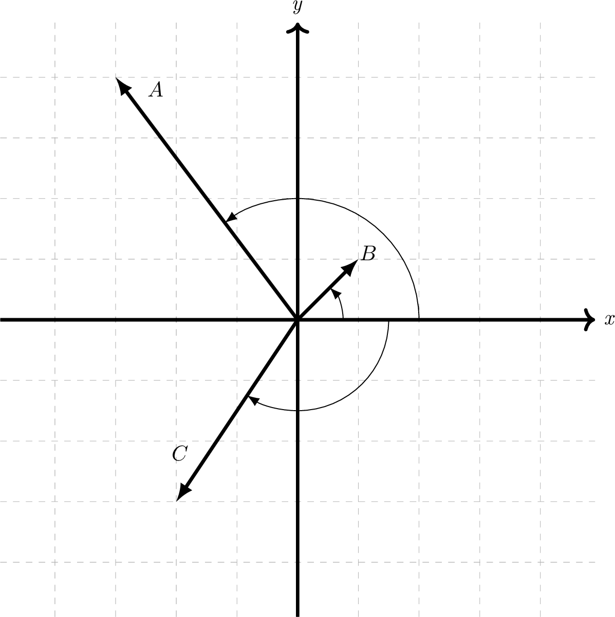
Figure 4.8: Three vectors labelled \(A\), \(B\) and \(C\).

The answer is in this⁴⁶ footnote.

4.5 Converting between Cartesian and Polar notations

As you may have already noticed there should be a fairly straightforward way to convert forwards and backwards between polar and rectangular notations. Clearly they are both valid ways to describe a vector so every vector should have both a polar and rectangular representation.

In order to convert between the two formats you need to use a little trigonometry, and Pythagoras’ theorem.

Let’s consider a vector \(\underline{v}\) which we write in both notations. So,

• Polar notation: \(\underline{v}=(r,\theta)\), and also
• Rectangular notation: \(\underline{v}=\begin{pmatrix}x \\ y \end{pmatrix}\)

4.5.1 Polar to Rectangular

The easiest direction for conversion is probably Polar to Rectangular. In Figure 4.9 below you can see that a vector with labelled polar notation \((r,\theta)\) has been drawn. Additionally a right-angled triangle has been drawn underneath this vector.

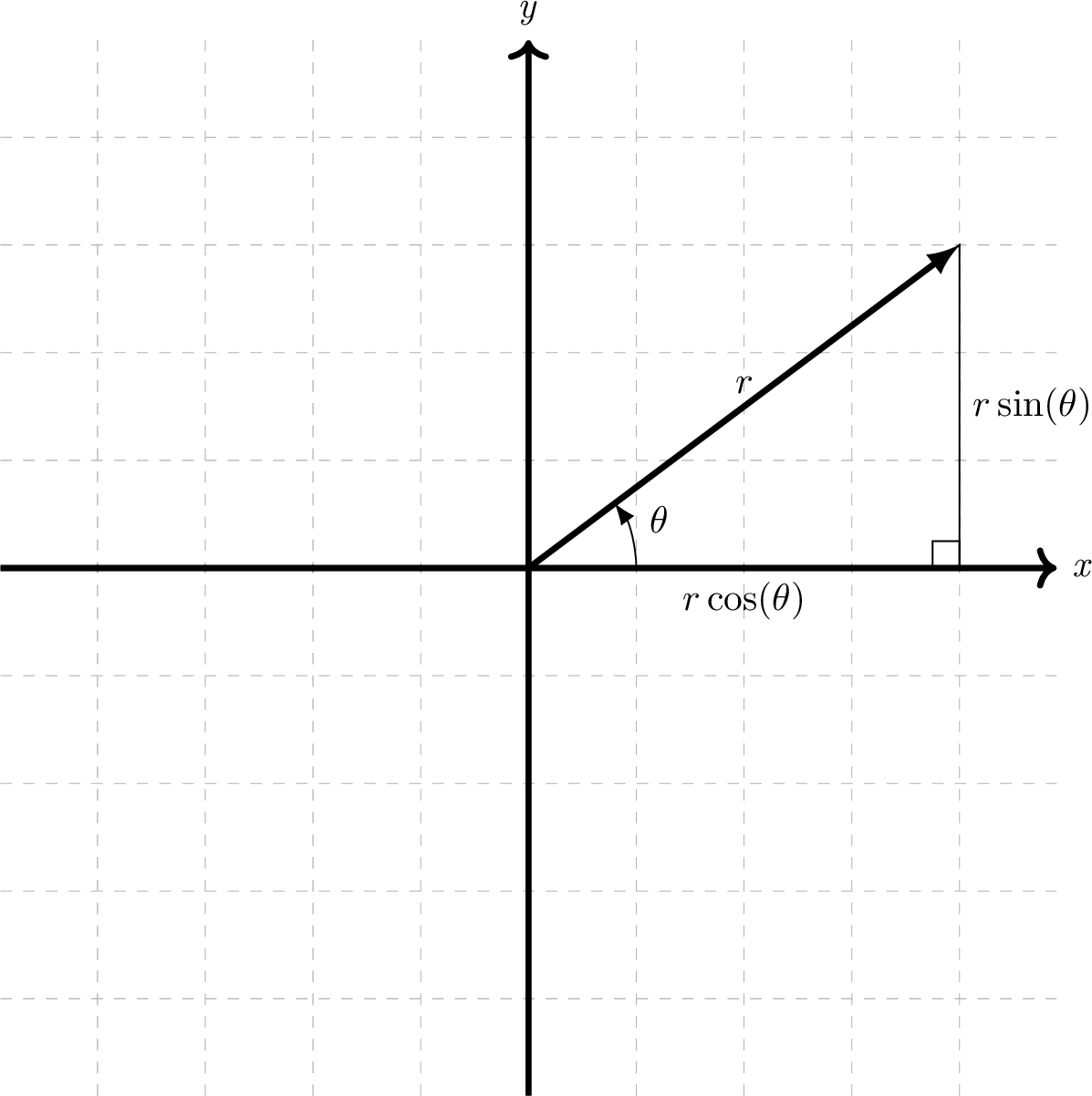
Figure 4.9: How to convert polar to rectangular notation

Basic trigonometry has been performed in the above diagram to label the \(x\) and \(y\) lengths of the triangle drawn. This means there is a straightforward conversion formula. If you would like to see the trigonometry behind this then here is a video, otherwise you can skip to the formula below.

Alternative direct video link:

https://gcu.planetestream.com/View.aspx?id=5994~4B~dmaaP9m7

Standard conversion formula:

\[\begin{equation} \begin{matrix} \textrm{(Polar notation) } & (r,\theta) \\ & \downarrow \\ \textrm{(Rectangular notation) } & (r \cos(\theta),r \sin(\theta)) \end{matrix} \tag{4.1} \end{equation}\]

This picture method works if the vector lives in the top-right quadrant on the graph, but what happens if the angle \(\theta\) isn’t between \(0^{\circ}\) and \(90^{\circ}\)?

The great news is that we don’t need to worry, as these formulae with \(\cos(\theta)\) and \(\sin(\theta)\) also work outside this range.

Here is a video to help you see this conversion working for the angle \(120^{\circ}\):

Alternative direct video link:

https://gcu.planetestream.com/View.aspx?id=5995~4C~FapLz8xu

In the video we had \(\theta=120^{\circ}\) and so, since \(\cos(120^{\circ})=-0.5\),

\[r \cos(\theta) = r \cos(120^{\circ}) = -0.5r \]

i.e. the \(x\) co-ordinate becomes negative, which is what was expected for an angle of \(120^{\circ}\). These conversion formulae, using \(r\cos(\theta)\) and \(r\sin(\theta)\), work for all \(r\) and all \(\theta\).

4.5.2 Rectangular to Polar

This conversion is also not super difficult, but it is a little trickier to make sure you get the angle correct.

We imagine this time starting with a vector with rectangular notation \((x,y)\) and want to calculate its polar version \((r,\theta)\).

The answer is actually very easy if \(x=0\) because then the vector either points vertically upwards⁴⁷ or vertically downwards⁴⁸ and the angle will be \(90^{\circ}\) or \(-90^{\circ}\) respectively. The length \(r\) will just be the size⁴⁹ of \(y\).

We can solve the cases where \(y=0\) very similarly (the angle will be \(0^{\circ}\) or \(180^{\circ}\)).

So we will only need the calculations below if \(x\) and \(y\) are not zero.

We start with a sketch from which its obvious we can use Pythagoras’ theorem to find \(r\) (Figure 4.10):

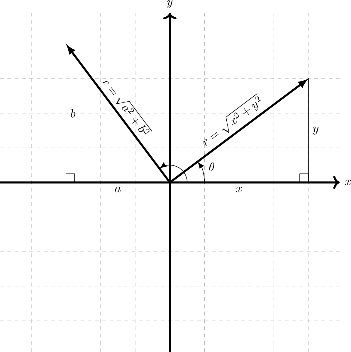
Figure 4.10: How to use Pythagoras to find vector length

Just looking at the vector lengths in this diagram it’s clear that we can just square the two values, add them and then square root the answer to use Pythagoras to find the length of the vector. This even works in the case above where \(a\) is negative, because \(a^2\) will be positive anyway.

Standard formula for polar length, \(r\), from rectangular notation \((x,y)\):

\[ r = \sqrt{x^2+y^2} \]

The difficulty comes with making sure we measure the correct angle in the diagram. Looking at the triangle drawn in the top-right, with side lengths \(x\) and \(y\), we know the formula for the angle \(\theta\) will be \[ \theta = \tan^{-1}\left(\frac{y}{x} \right), \quad \textrm{sometimes also called }\arctan\left(\frac{y}{x} \right). \]

However, calculating \(\tan^{-1}\left(\frac{b}{a} \right)\) for the triangle in the top-left may not find the angle desired because most calculators give the answer to \(\tan^{-1}\) that lies between \(-90^{\circ}\) and \(90^{\circ}\), and we want an angle that lies outside this range, at approximately \(120^{\circ}\). There are many valid approaches but perhaps the cleanest is to always convert the sides of the right-angled triangle into lengths (i.e. turn negative numbers positive) and consider this picture:

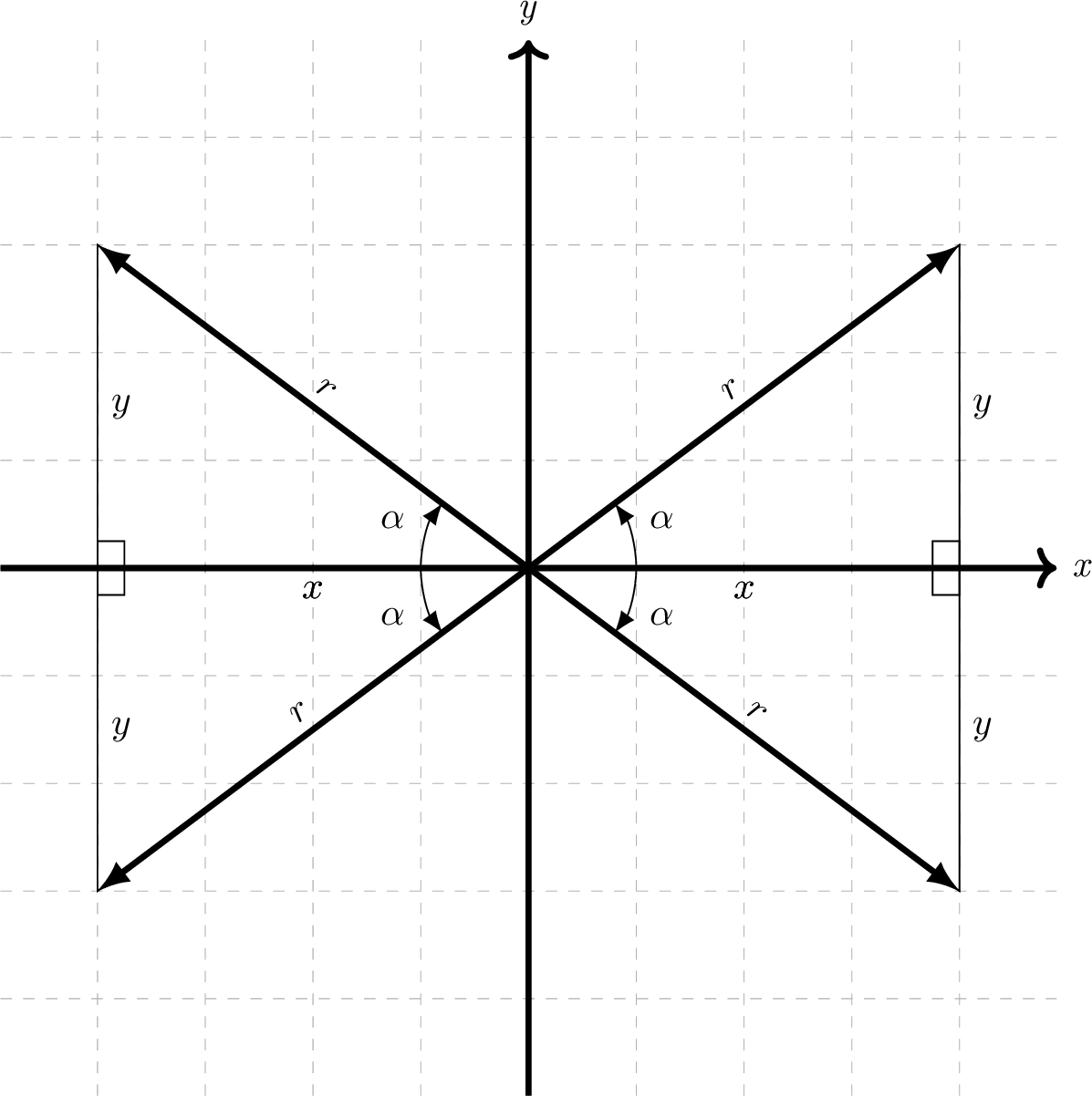
Figure 4.11: Using \(\tan^{-1}\left(\frac{|y|}{|x|}\right)\) always returns one of these four positive \(\alpha\).

Notice in Figure 4.11 there are four vectors drawn, and four triangles (each with sides \(x\) and \(y\)) and that the angle labelled \(\alpha\) is always the angle created between a vector and the \(x\)-axis. In this picture four identical angles are all labelled \(\alpha\) and they are the positive angle obtained if you calculate \[ \alpha= \tan^{-1}\left(\frac{|y|}{|x|}\right)\]

where the notation \(|y|\) and \(|x|\) just means to take the size⁵⁰ of \(y\) and \(x\) respectively, basically just ignoring their sign. e.g. \(|4|=4, |-2|=2, |1|=1, |-17|=17\) etc…

To work out the correct angle \(\theta\) for the polar notation, isn’t too difficult once you have \(\alpha.\)

The formula for the polar angle \(\theta\) from rectangular notation \((x,y)\) can be found by first calculating

\[ \alpha= \tan^{-1}\left(\frac{|y|}{|x|}\right) \]

Then, based on where the vector (starting from the origin) lives…

• In the top-right corner \(\theta=\alpha\) already.
• In the bottom-right corner \(\theta=-\alpha\),
• In the bottom-left corner \(\theta=-180^{\circ}+\alpha\),
• In the top-left corner \(\theta=180^{\circ}-\alpha\).

It’s easiest to just draw a sketch like Figure 4.11 above, to recreate these rather than try and memorize them.

To work these out manually just remember that the negative \(x\)-axis is \(180^{\circ}\) around from the positive \(x\)-axis.

Link to Numbas on the web

Link to Numbas on the web

4.6 Vector addition and subtraction

Now that we’ve invented a whole new type of object, a vector, and we’ve covered in detail the ways to represent vectors, we are allowed to decide what it means to add two vectors together, or subtract two vectors from each other. Luckily for us, mathematicians who first worked with vectors have already agreed upon a very useful meaning which allows us to solve a wide range of problems without getting too complicated.

If we recall that we can think of vectors as describing movements, then adding two vectors represents doing one movement after the other.

So if vector \(\underline{v}=\begin{pmatrix} 2 \\ -3 \end{pmatrix}\) and vector \(\underline{w}=\begin{pmatrix} -5 \\ 4 \end{pmatrix}\) so that

• \(\underline{v}\) represents moving right \(2\) and down \(3\), and
• \(\underline{w}\) represents moving left \(5\) and up \(4\)

then we say that \(\underline{v}+\underline{w}\) represents

‘moving right \(2\) and down \(3\)’ then ‘moving left \(5\) and up \(4\).’

Geometrically it can be calculated by drawing the vector \(\underline{w}\) to start at the end of vector \(\underline{v}\) like the picture in Figure 4.12. Notice that the vector \(\underline{w}\) has been drawn to start at the end of \(\underline{v}\).

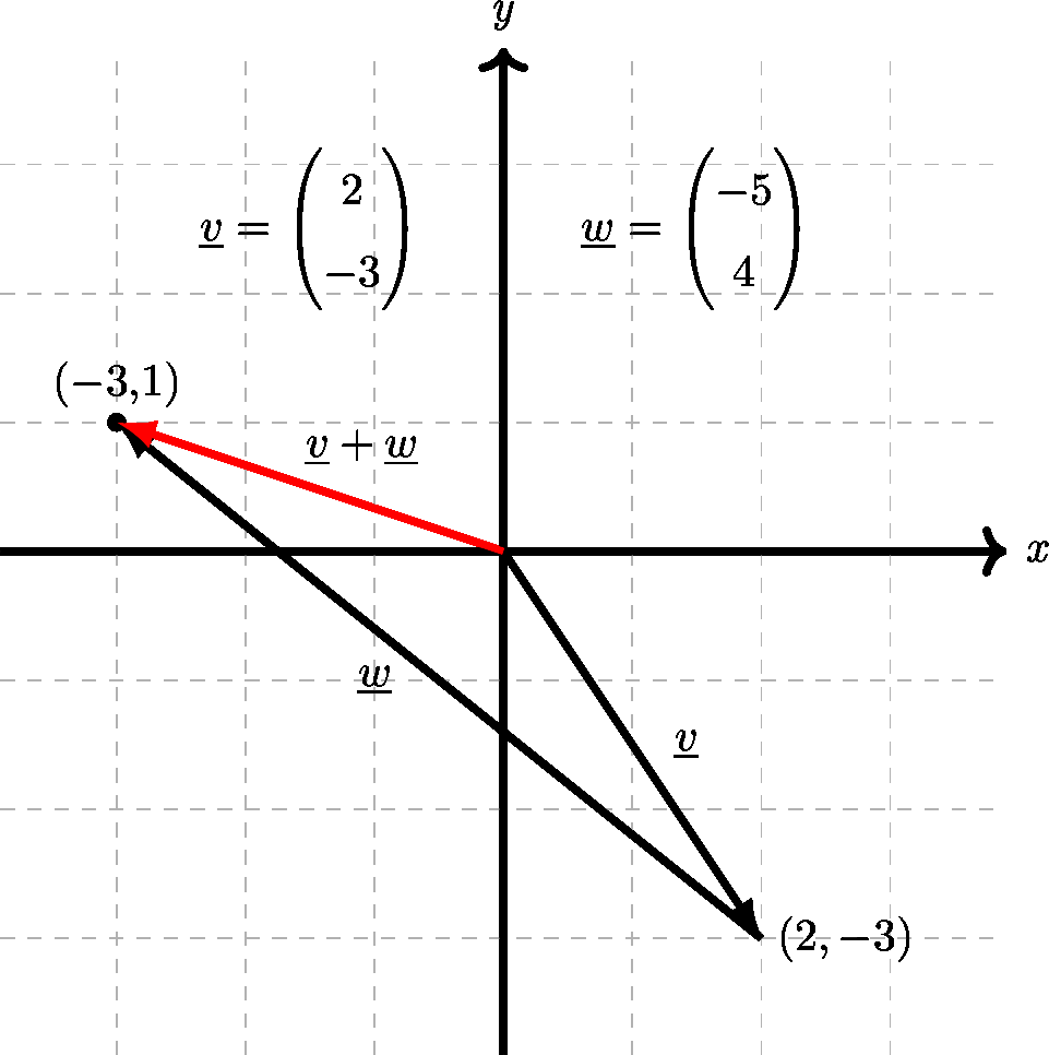
Figure 4.12: Illustration of geometry of vector addition.

Thankfully, algebraically it’s even easier, if the vectors are in rectangular notation, you just add the corresponding components like this:

\[\begin{align*} \underline{v}+\underline{w} & = \begin{pmatrix} 2 \\ -3 \end{pmatrix} + \begin{pmatrix} -5 \\ 4 \end{pmatrix} \\ & = \begin{pmatrix} (2)+(-5) \\ (-3)+(4) \end{pmatrix} = \begin{pmatrix} -3 \\ 1 \end{pmatrix} \end{align*}\]

So \(\underline{v}+\underline{w}\) is the vector which represents moving \(3\) left and \(1\) up, i.e. the net effect of doing \(\underline{v}\) and then \(\underline{w}\)⁵¹.

So the general formula for adding vectors just looks like this:

\[\begin{equation} \begin{pmatrix} a \\ b \end{pmatrix} + \begin{pmatrix} c \\ d \end{pmatrix} = \begin{pmatrix} a+c \\ b+d \end{pmatrix} \tag{4.2} \end{equation}\]

Subtraction works in exactly the same way, you can either think of \(\underline{v}-\underline{w}\) as \(\underline{v}+(-\underline{w})\) or use the formula: \[\begin{equation} \begin{pmatrix} a \\ b \end{pmatrix} - \begin{pmatrix} c \\ d \end{pmatrix} = \begin{pmatrix} a-c \\ b-d \end{pmatrix} \tag{4.3} \end{equation}\]

If you begin with your vectors in polar notation, however, then it’s much trickier to add them together. Indeed the easiest method is normally to convert them first into another notation (like rectangular) and then perform the calculation.

The examples below can be used to practice adding and subtracting vectors. You can generate a new random example using the button below each question. In this example, the Reveal answers button will also show you how to do the question if you are stuck.

Link to Numbas on the web

Link to Numbas on the web

4.7 Multiplying a vector by a scalar

Here we’re combining two terms we have learnt in this chapter. Recall that a scalar is just another name for a constant, a single-value or number (in contrast to a vector which includes a direction). So if we have a vector \(\underline{w}\) then examples of multiplying by a scalar would include \[ 2\underline{w}, 3\underline{w}, -\underline{w}, 3.4 \underline{w}, -\sqrt{7}w \] Note, that in the third example, just like when performing algebra normally \(-\underline{w}\) is just a short version of \(-1\times \underline{w}\).

Since the idea of multiplication is really just repeated addition, so that multiplying something by \(2\) is the same as adding it to itself, it’s not a surprise that multiplying a vector by a scalar is also pretty easy.

If you’ve been wondering until now why scalars are called scalar… then you’re about to see. Multiplication by scalars has the effect of scaling the vector, in the sense that scaling is used to change the size of an image. Scaling by a factor of \(2\) means to double the size, scaling by \(3\) means to triple the size, etc…

As a simple example, if \(\underline{w}=\begin{pmatrix} -1 \\ 2 \end{pmatrix}\) then \(5\underline{w}=\begin{pmatrix} -5 \\ 10 \end{pmatrix}\).

The standard formula for scalar multiplication looks as follows. If we call our scalar \(k\) then in rectangular format \[\begin{equation} k \times \begin{pmatrix} x \\ y \end{pmatrix} = \begin{pmatrix} k \times x \\ k\times y \end{pmatrix} \tag{4.4} \end{equation}\]

Geometrically, it’s also quite easy to see how scaling works. First, in Figure 4.13, some examples to show how scaling works for simple positive multiples.

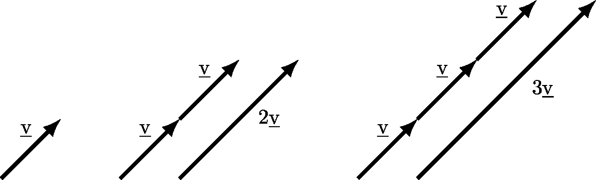
Figure 4.13: Illustration of geometry of vector addition.

Next, in Figure 4.14, we see that the negative of a vector just reverses the direction, and fractional multiples behave as expected. So \(1.5\underline{v}\) is \(50\%\) longer than \(\underline{v}\).

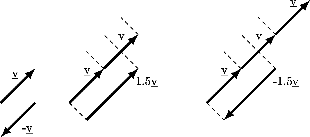
Figure 4.14: Illustration of geometry of scalar multiplication of a vector.

In polar notation it’s also fairly easy, since scaling a vector never actually changes the direction of the vector, except when we multiply by a negative scalar. In which case the direction is completely reversed. Thus a vector with angle \(\theta=30^{\circ}\) when multiplied by \(-1\) is completely reversed and now has angle \(-150^{\circ}\). Or a vector that begins with angle \(\theta=-50^{\circ}\) is totally reversed and becomes a new vector with an angle of \(130^{\circ}\). The precise formula depends on whether the original \(\theta\) was negative or positive. Notice also that the length of a vector is doubled when it is multiplied by \(2\) or is multiplied by \(-2\), it’s just the angle also changes in the latter.

Multiplying vectors by scalars in polar form, is best visualized geometrically, but the formulae also look like this:

If \(k>0\) then

\[ k \times (r,\theta) = (k\times r, \theta). \]

But if \(k<0\), then first recall that \(-k=|k|\) is the positive scaling factor, and

\[ k \times (r,\theta) = (|k|\times r, \theta+180^{\circ}\textrm{ or }\theta-180^{\circ}) \]

which one of the two angles above is correct, is whichever one fits in the standard range between \(-180^{\circ}\) and \(180^{\circ}\).

It’s not recommended to try and memorize this formula, best to get a geometric understanding by trying some examples.

Practice

In Figure 4.15, which of the four labelled vectors represents \(\underline{v}\) and which one represents \(-1 \times \underline{v}\), i.e. \(-\underline{v}\)?

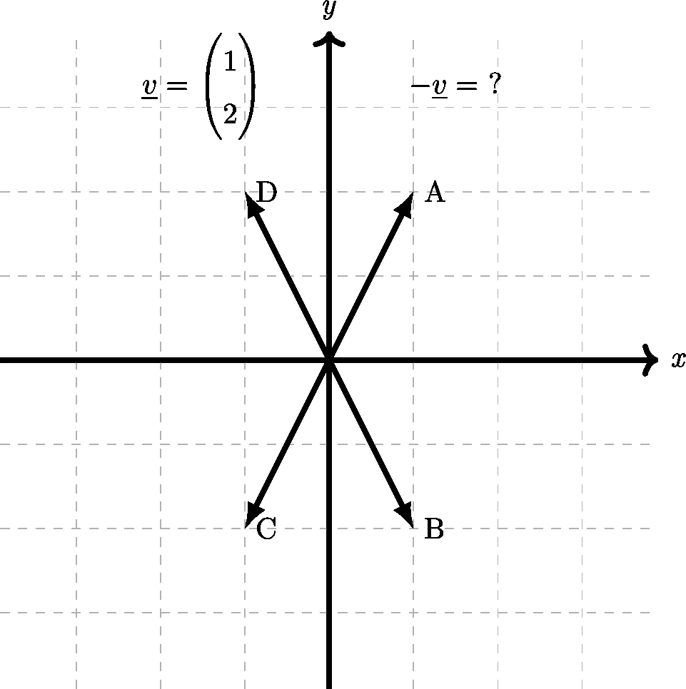
Figure 4.15: Four vectors, but which is \(-\underline{v}\)?

Next, a scaled vector. The (shortest) black vector is \(\underline{v}\), which of the other vectors is \(3\underline{v}\)?

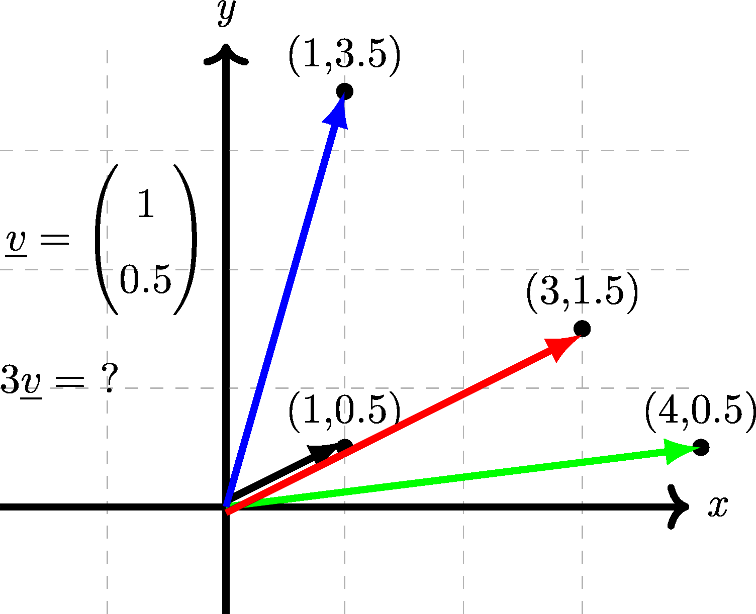
Figure 4.16: Which one is \(3\underline{v}\)?

Answers⁵²

4.8 Relative position vectors

One natural use of vectors is to represent locations of objects in a diagram, like in force diagrams. In such cases objects are often described by labelling their locations and the edges between such points can be represented as vectors.

A vector that describes the displacement between two positions in space is called a relative position vector.

e.g. if a point \(P\) is located at \((3,1)\) and point \(Q\) is located at \((-1,3)\) then, the position vector of \(Q\) relative to \(P\) is written \(\overrightarrow{PQ}\) and calculated by subtracting the co-ordinates of \(P\) from \(Q\). Alternatively, you can subtract \(\overrightarrow{OP}\) from \(\overrightarrow{OQ}\) like this:

\[ \overrightarrow{PQ} = \begin{pmatrix} -1 \\ 3\end{pmatrix} - \begin{pmatrix} 3 \\ 1\end{pmatrix} = \begin{pmatrix} -4 \\ 2\end{pmatrix}. \]

The \(\overrightarrow{PQ}\) notation is used, because a directed line (starting at \(P\)) joining \(P\) to \(Q\) will match the vector in direction and length.

Recall: this arrow notation to signify a vector is one of the alternatives to underlining a vector. It is almost always used in this kind of example where you have locations described by letters.

As previously, it is not important to learn the formula for the relative position vector, it is better for future applications if you can work it out by remembering that the relative position vector of \(Q\) from \(P\) is the vector required by someone who starts at \(P\) who wants to travel to \(Q\).

In the examples above \(P=(3,1)\) and \(Q=(-1,3)\) so to reach \(Q\) from \(P\) requires:

• Subtracting \(4\) from the \(x\)-coordinate (notice \(-4=(-1)-(3)\)), and
• Adding \(2\) to the \(y\)-coordinate (notice \(2=(3)-(1)\)).

Here is that same example, shown in geometric form, where it is easier to see the vector \(\overrightarrow{PQ}\):

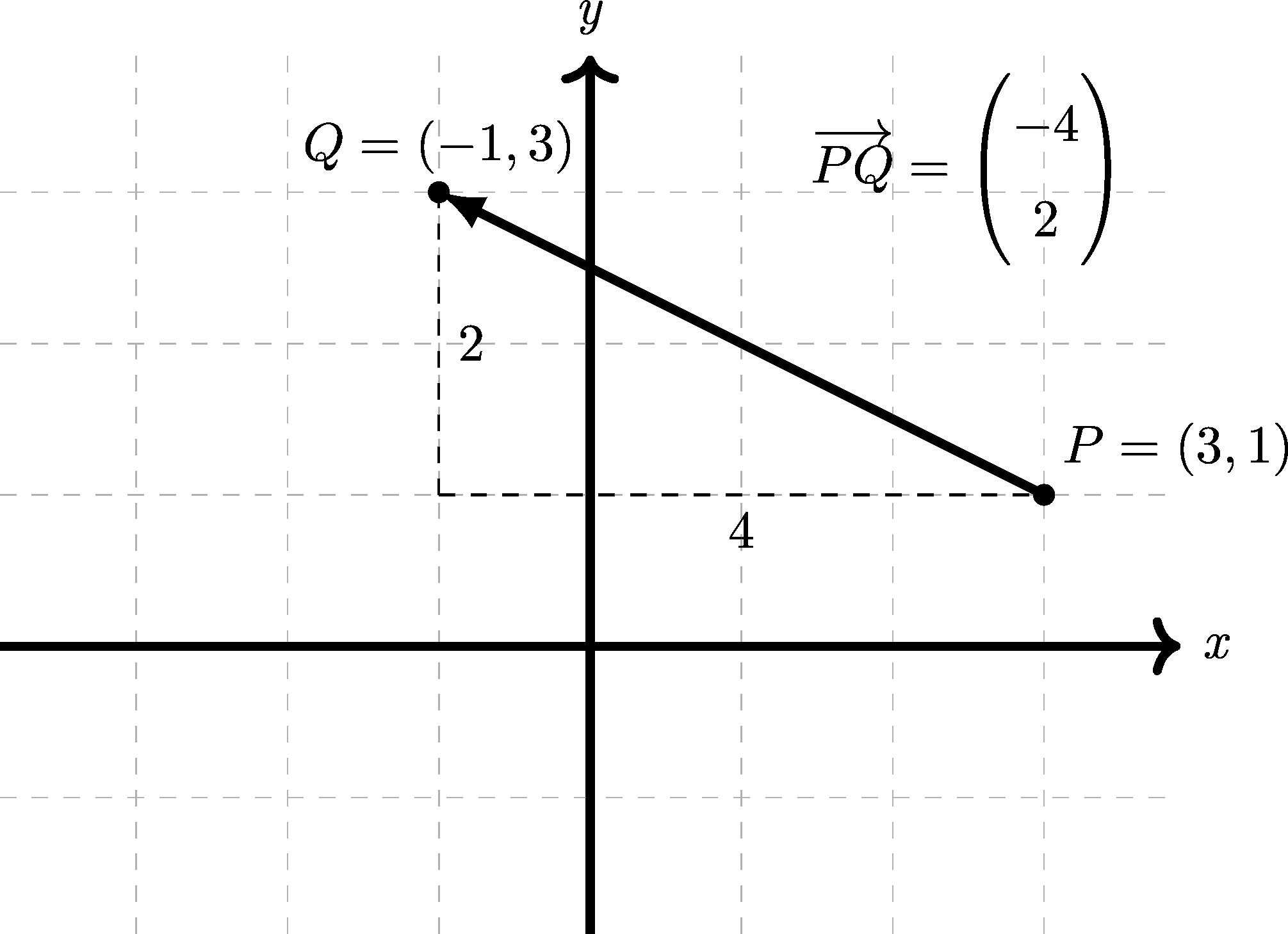
Figure 4.17: Illustration of a relative position vector. Here, the position vector of \(Q\) relative to \(P\) is written \(\overrightarrow{PQ}\).

It is again hopefully clear that the calculation of a relative position vector is quite straightforward when vectors are written in rectangular format. Since this calculation is a subtraction the difficulty in doing this with vectors written in polar notation is the same as it was in Section 4.6.

4.9 The \(\underline{i}\), \(\underline{j}\) notation for vectors

Introduction of a final alternative rectangular notation has been saved until now as it really is just a completely equivalent alternative to the previously introduced Rectangular/Cartesian format.

Definition of the \(\underline{i}\), \(\underline{j}\) vectors.

For this notation we introduce two special vectors: \[ \underline{i} = \begin{pmatrix} 1 \\ 0 \end{pmatrix} \textrm{ and } \underline{j} = \begin{pmatrix} 0 \\ 1 \end{pmatrix} \]

We have already introduced the standard rules for addition, subtraction and scalar multiplication of vectors. So it only remains for us to appreciate how these rules manifest in this new \(\underline{i}\), \(\underline{j}\) notation. One reason this notation is popular is because it allows the \(\underline{i}\) and \(\underline{j}\) to be treated much like we treat unknowns when we perform algebra.

Firstly, it’s very easy to convert from rectangular to \(\underline{i}\), \(\underline{j}\) notation:

\[ \begin{pmatrix} 3 \\ 7 \end{pmatrix} = 3 \begin{pmatrix} 1 \\ 0 \end{pmatrix} + 7\begin{pmatrix} 0 \\ 1 \end{pmatrix} = 3\underline{i}+7\underline{j}\] or in general \[ \begin{pmatrix} x \\ y \end{pmatrix} = x \begin{pmatrix} 1 \\ 0 \end{pmatrix} + y\begin{pmatrix} 0 \\ 1 \end{pmatrix} = x\underline{i}+y\underline{j}\] for any values (positive, zero, or negative) of \(x\) and \(y\).

• The constant in front of the \(\underline{i}\) vector corresponds to the \(x\)-coordinate.
• The constant in front of the \(\underline{j}\) vector corresponds to the \(y\)-coordinate.

You can do addition and subtraction using this notation in a standard algebraic way, by grouping the \(\underline{i}\) terms and \(\underline{j}\) terms separately, just as you would two different letters in algebra.

For example,

\[ \left(2\underline{i}+3\underline{j}\right) + \left(3\underline{i}-9\underline{j}\right) = 5\underline{i}-6\underline{j} \]

or if \(\underline{v}=3\underline{i}+\underline{j}\) and \(\underline{w}=-\underline{i}+7\underline{j}\) then

\[\begin{align*} 2\underline{v}-3\underline{w} &= 2\left(3\underline{i}+\underline{j}\right)-3\left(-\underline{i}+7\underline{j}\right) \\ &= \left(6\underline{i}+2\underline{j}\right) - \left(-3\underline{i}+21\underline{j}\right) \\ &= 9\underline{i}-19\underline{j} \end{align*}\]

This notation is very often used in textbooks and resources as a way to avoid the slightly more space-consuming rectangular column vector notation which can span multiple lines of text. However, obviously some users may also just prefer it.

Practice

Match up these five vectors written in matrix notation with the \(\underline{i},\underline{j}\) vectors below.

The column vector formats:

1. \(\begin{pmatrix} 3 \\ 4 \end{pmatrix}\)
2. \(\begin{pmatrix} 0 \\ 2 \end{pmatrix}\)
3. \(\begin{pmatrix} 2 \\ 0 \end{pmatrix}\)
4. \(\begin{pmatrix} 4 \\ 3 \end{pmatrix}\)
5. \(\begin{pmatrix} 4 \\ -3 \end{pmatrix}\)

The \(\underline{i},\underline{j}\) notation:

1. \(4 \underline{i} + 3 \underline{j}\)
2. \(2 \underline{i}\)
3. \(3 \underline{i} + 4 \underline{j}\)
4. \(4 \underline{i} - 3 \underline{j}\)
5. \(2\underline{j}\)

Answers⁵³

4.10 The Scalar (or Dot) product of two vectors

Having discussed multiplying vectors by scalars in Section 4.7, one could naturally ask the question of whether vectors can also be multiplied by each other.

Since vectors were a new mathematical object, the creators were free to decide what this multiplication is designed to represent and mean. The result of the study was that there are actually two different useful ways to define the multiplication of one vector with another vector. This section (Section 4.10) will discuss the first of these:

• The Scalar Product (also known as the Dot (\(\cdot\)) Product);
• The Vector Product (also known as the Cross (\(\times\)) Product) will be discussed in Section 4.13

Each of these products has two names(!) because one name describes what sort of output you get, and the alternative name describes the symbol used to denote the multiplication. We cannot just use \(\times\) like we have always done in algebra, because we are going to have two different ways to define multiplication.

Unsurprisingly, the Dot Product will use a dot like this, \(\cdot\), and the Cross Product (see later) will use a cross, like this, \(\times\). But because their other names are more helpful we shall stick to calling them the Scalar⁵⁴ and Vector⁵⁵ products for the time being.

The Scalar Product is a way to multiply two vectors which gives a scalar as its output. The easy formula definition available in rectangular notation is as follows.

If \(\underline{v}=\begin{pmatrix} x \\ y \end{pmatrix}\) and \(\underline{w}=\begin{pmatrix} a \\ b \end{pmatrix}\) then \[\begin{equation*} \underline{v}\cdot\underline{w} = xa+yb \tag{4.5} \end{equation*}\]

Let’s see a few examples involving numbers, from which it should be obvious how to calculate the Scalar Product.

For vectors \(\underline{v}=\begin{pmatrix}8\\-2 \end{pmatrix}\) and \(\underline{w}=\begin{pmatrix}3\\4 \end{pmatrix}\) their Scalar Product is

\[ \underline{v}\cdot\underline{w} = \begin{pmatrix}8\\-2 \end{pmatrix} \cdot \begin{pmatrix}3\\4 \end{pmatrix}= 8 \times 3 + (-2)\times 4 = 16. \]

For vectors \(\underline{a}=\begin{pmatrix}-1\\4 \end{pmatrix}\) and \(\underline{b}=\begin{pmatrix}-2\\7 \end{pmatrix}\) their Scalar Product is

\[ \underline{a}\cdot\underline{b} = \begin{pmatrix}-1\\4 \end{pmatrix} \cdot \begin{pmatrix}-2\\7 \end{pmatrix}= (-1) \times (-2) + 4\times 7 = 30. \]

For vectors \(\underline{v}_1=\begin{pmatrix}3\\1 \end{pmatrix}\) and \(\underline{v}_2=\begin{pmatrix}-1\\3 \end{pmatrix}\) their Scalar Product is

\[ \underline{v_1}\cdot\underline{v_2} = \begin{pmatrix}3\\1 \end{pmatrix} \cdot \begin{pmatrix}-1\\3 \end{pmatrix}= 3 \times (-1) + 1\times 3 = 0. \]

It’s worth noting in this final example we have used subscripts rather than different letters to name our vectors. This is a very typical approach because when working with vectors you can often quickly run out of new letters, so it’s easier to use just one letter like \(\underline{v}\) and use subscripts to name them differently.

There is an alternative definition of the Scalar Product, which is useful for finding the angle between two vectors, but not very useful for actually calculating the Dot Product:

\[\begin{equation} \underline{v}\cdot\underline{w} = \operatorname{length}(\underline{v})\times \operatorname{length}(\underline{w})\times \cos(\theta) \tag{4.6} \end{equation}\]

where \(\theta\) is the angle between the vectors \(\underline{v}\) and \(\underline{w}\).

Authors often use the notation \(|\underline{v}|\) for \(\operatorname{length}(\underline{v})\) so this formula is often written: \[\begin{equation} \underline{v}\cdot\underline{w} = |\underline{v}| |\underline{w}| \cos(\theta). \tag{4.7} \end{equation}\]

If we have written our vector in Polar format then the length is just called \(r\). If we have our vector in Rectangular notation then we need to use Pythagoras to work out its length.

As stated above, this formula is not generally useful for actually finding the Scalar Product of two vectors because the formula given before is so easy to use. Additionally we don’t normally know the angle between two vectors. However, as we shall see in Section 4.11 we can use this new formula to work out the angle between two vectors. By the angle between two vectors, we just mean the angle you create if you draw both vectors starting at the same point and measure the gap from the first to the second vector, e.g.

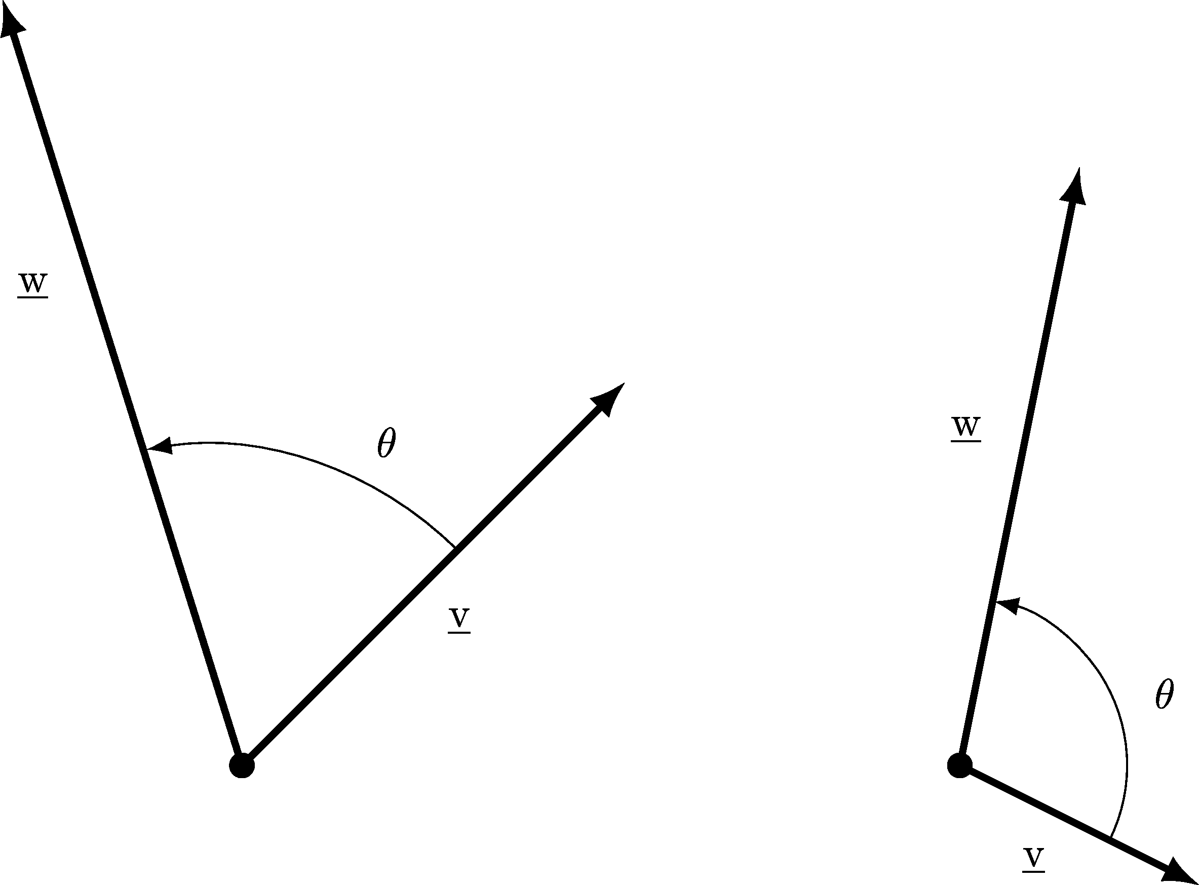
Figure 4.18: Two examples of the angle between two vectors, called \(\theta\) in the Scalar Product formula.

As a final aside, while you will generally use the Rectangular format to work out a Scalar Product, if you do happen to start with two vectors in Polar format, e.g. \(\underline{v}=(r_1,\theta_1)\) and \(\underline{w}=(r_2,\theta_2)\) then finding the Scalar Product is actually pretty easy. We know that \(\operatorname{length}(\underline{v})=r_1\) and \(\operatorname{length}(\underline{w})=r_2\). And the angle between the two vectors will simply be \(\theta_2-\theta_1\) (draw a little sketch if you want). So, occasionally this version of the formula is useful:

\[ (r_1,\theta_1)\cdot(r_2,\theta_2) = r_1 r_2 \cos(\theta_2-\theta_1). \]

In the next section we shall discover why the Scalar Product is so useful.

Some examples to practice calculating Scalar Products will appear in the examples at the end of the notes in Section 7.

4.11 Applications of the Scalar Product

The Scalar Product calculation has many useful applications, below we shall discuss just four of these, although there are others.

4.11.1 How to find the angle between two vectors

Given two vectors, \(\underline{v}\) and \(\underline{w}\), we can use the Scalar Product to quickly find the angle between them. If you imagine drawing the two vectors both starting from the same point (see Figure 4.18 for two such examples) this is the angle we shall try to find.

There are four steps:

• Starting in Rectangular format, use the simple Scalar Product formula to calculate \(\underline{v}\cdot\underline{w}\) (see (4.5));
• Find the lengths of the vectors (using Pythagoras);
• Re-arrange the \(\underline{v}\cdot\underline{w} = \operatorname{length}(\underline{v})\times \operatorname{length}(\underline{w})\times \cos(\theta)\) formula to find \(\cos(\theta)\);
• Use inverse cosine to find \(\theta\).

Let’s try it with \(\underline{v}=\begin{pmatrix} 2 \\ -1 \end{pmatrix}\) and \(\underline{w}=\begin{pmatrix} 1 \\ 5 \end{pmatrix}\)

First,

\[ \underline{v}\cdot\underline{w} = \begin{pmatrix}2\\-1 \end{pmatrix} \cdot \begin{pmatrix}1\\5 \end{pmatrix}= 2 \times 1 + (-1)\times 5 = -3. \]

Next we find the vectors’ lengths,

\[ \operatorname{length}(\underline{v}) = |\underline{v}| = \sqrt{2^2 + (-1)^2} = \sqrt{5}, \] and \[ \operatorname{length}(\underline{w}) = |\underline{w}| = \sqrt{1^2 + 5^2} = \sqrt{26}. \] Substituting these values into either of the formulae above ((4.6) or (4.7)), \[ -3 = \sqrt{5}\sqrt{26} \cos(\theta),\] which can be rearranged to say \[ \cos(\theta) = \frac{-3}{\sqrt{5}\sqrt{26}} \approx -0.2631. \]

Finally we use \(\cos^{-1}\) to get

\[ \theta = \cos^{-1}(-0.2631) \approx 105.255^{\circ}. \]

This is our angle from \(\underline{v}\) to \(\underline{w}\). Try sketching the vectors yourself and verify that the angle is indeed slightly more than a right-angle. In fact, this example is the right-most example in Figure 4.18!

A minor note is that the angle \(360^{\circ}-\theta\) is always the angle between the vectors if you consider \(\underline{w}\) to \(\underline{v}\) rather than \(\underline{v}\) to \(\underline{w}\).

4.11.2 How to check if two vectors form a right-angle

If two vectors form a right-angle then the technical term used is that they are orthogonal (to each other)⁵⁶.

Checking for orthogonality is actually much easier than finding the angle between two vectors. Recall that if the angle \(\theta=90^{\circ}\) then

\[ \cos(\theta) = \cos(90^{\circ}) = 0. \]

So if we look at the complicated Scalar Product formula ((4.6)):

\[\begin{equation*} \underline{v}\cdot\underline{w} = \operatorname{length}(\underline{v})\times \operatorname{length}(\underline{w})\times \cos(\theta), \tag{4.8} \end{equation*}\]

we notice that if the angle between vectors \(\underline{v}\) and \(\underline{w}\) is \(\theta=90^{\circ}\) then \(\cos(\theta)=0\) and the right-hand side of the equation will equal \(0\)! So it follows that \(\underline{v}\cdot\underline{w}=0\).

This means that whenever two vectors form a \(90^{\circ}\) angle, then their Scalar Product will be zero!

Even better is the news that by looking at the right-hand side of (4.8) the only way for the right-hand side to be equal to zero is if \(\cos(\theta)=0\) unless we’ve stupidly started with a vector of length \(0\) (which doesn’t really make any angles)⁵⁷. So as long as neither of our vectors is just a vector of zeroes, then the only way to get \(\underline{v}\cdot\underline{w}=0\) is via an angle of \(90^{\circ}\) (or \(270^{\circ}\), if being picky, but that’s just \(90^{\circ}\) in disguise).

Our conclusion is that to check if two vectors are orthogonal, you just find their Scalar Product and check if it’s zero.

So the following two statements are actually saying exactly the same thing:

• \(\underline{v}\cdot\underline{w}=0\)
• \(\underline{v}\) and \(\underline{w}\) form a right-angle.

We can do a quick couple of examples:

Let’s try it with \(\underline{v}=\begin{pmatrix} 2 \\ -1 \end{pmatrix}\) and \(\underline{w}=\begin{pmatrix} 1 \\ 5 \end{pmatrix}\)

\[ \underline{v}\cdot\underline{w} = 2 \times 1 + (-1)\times 5 = -3 \neq 0. \]

So they are not orthogonal⁵⁸.

On the other hand, if we try \(\underline{a}=\begin{pmatrix} 3 \\ 1 \end{pmatrix}\) and \(\underline{b}=\begin{pmatrix} -1 \\ 3 \end{pmatrix}\), then

\[ \underline{a}\cdot\underline{b} = 3 \times (-1) + 1 \times 3 = 0 \]

so these two vectors are orthogonal. Sketch them and see it for yourself if you wish.

4.11.3 Finding the projection/component of a vector in a particular direction

Many applications of vectors to real-world force diagrams involve identifying what effect a known force has upon an object. Forces have both a strength⁵⁹ and a direction, however, and this direction can strongly effect how much of a force’s full strength acts on an object.

As an example, if you strike a nail with a hammer by hitting it directly flat on the head, then all of the force is acting in the direction of pushing the nail into your target. If, however, you strike the nail with an identical strength force, but only hit the nail at a \(45^{\circ}\) angle then some of your force is acting sideways and not assisting in pushing the nail into your target. That sideways force often results in you bending the nail, oops!

Another famous example is that of an object on a slope, sliding down under gravity. The steeper the slope the more of the gravitational force is aligned with the slope, and the shallower the slope the less effect the gravitational force has to move the object downhill. This process of calculating how much of the force acts in different directions is called resolving.

First a method you don’t need to learn for these notes, the standard trigonometry approach. Here is a typical diagram for an object on a slope with a labelled angle and gravitational force:

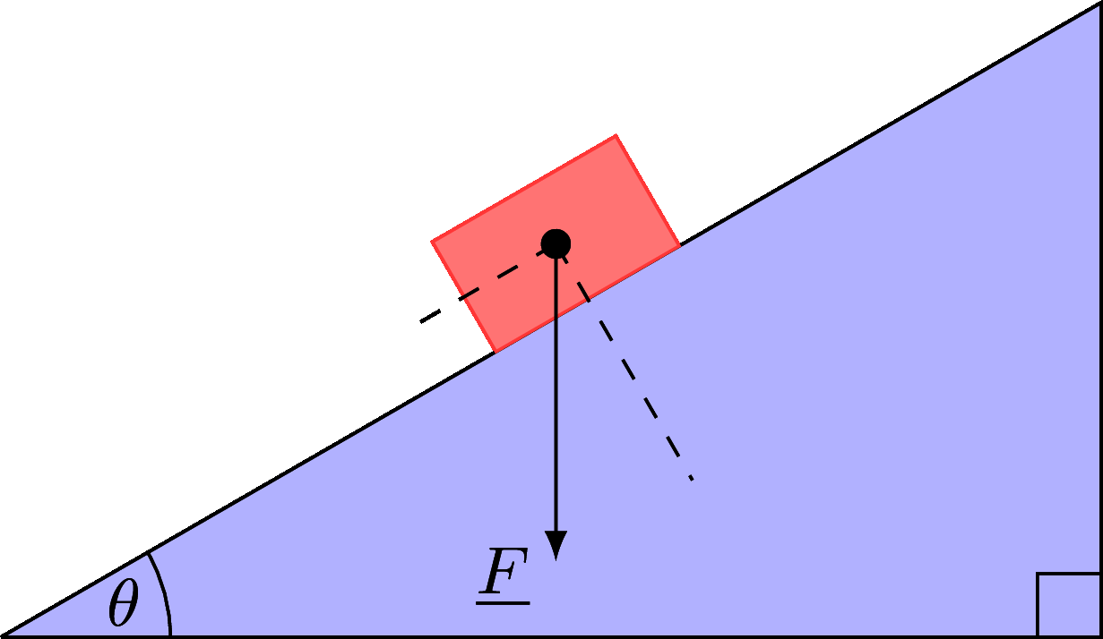
Figure 4.19: An object on a slope at angle \(\theta\), with a gravitational force labelled.

If we zoom into the object on the slope and label the angles, we can then use trigonometry to work out how much force is in each direction:

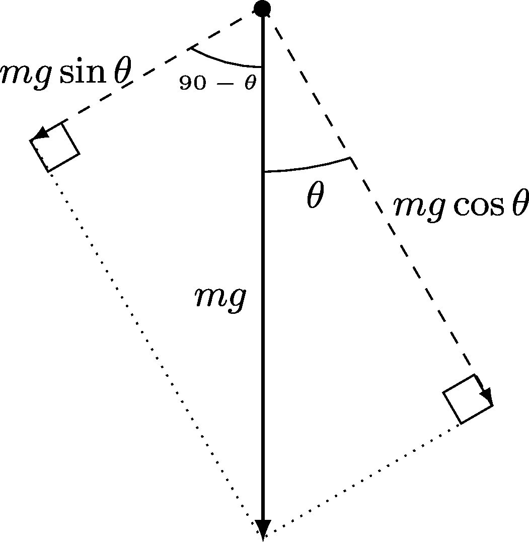
Figure 4.20: A zoom into the object on the slope with angles labelled.

Labelling these forces on the diagram we get the following version, showing how much of the force of \(mg\) Newtons is resolved in each direction:

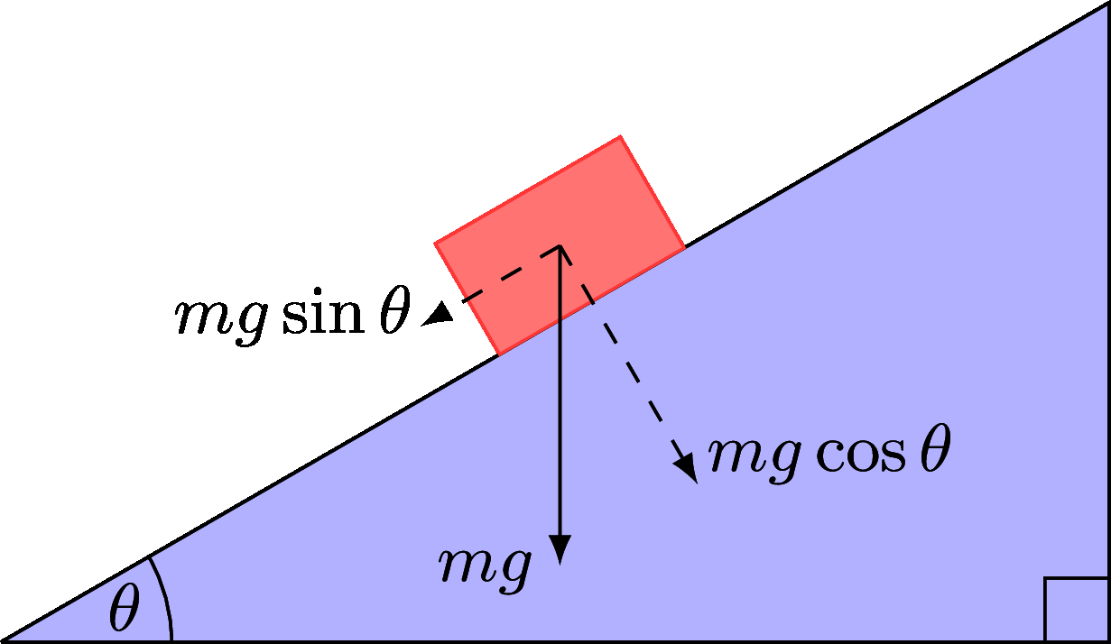
Figure 4.21: The object on the slope, with force size \(mg\) resolved into directions.

There is in fact a shortcut which skips using trigonometry, via our Scalar Product. This is the approach we shall learn here.

We define the Scalar projection of a force onto a line by taking a vector \(\underline{v}\) of length 1 in the direction of the line and then calculating:

\[ \underline{F}\cdot\underline{v}. \]

This projection of a force onto a line tells you how much of the force acts in this direction. (The same as resolving forces seen above.)

Definition of a unit vector

A vector which has length equal to \(1\) is known as a unit vector. We could have defined this earlier when defining length, but it wasn’t necessary.

For every possible direction there is always exactly only vector of length \(1\), so there are as many unit vectors as there are directions, i.e. infinity!

In a number of applications of scalar products, and vectors in general, we need to take a starting vector and change (or more technically scale) its length⁶⁰ to length \(1\). To do this you simply need to divide a vector by its length, or multiply it by the scalar \(\frac{1}{\textrm{length}}\).

e.g. given a vector length \(12\), multiplying the vector by \(\frac{1}{12}\) will create a new vector of length \(1\), without changing the vector’s direction.

To find how much of a force acts in a particular direction, we just find the Scalar Product of our force with a vector of length 1 (i.e. a unit vector) in the direction we care about.

Using the scalar product to resolve a force

If we consider exactly the same object on the slope from Figure 4.19, then we can find the size of the gravitational force acting down the slope by calculating the Scalar Product of the force, \(\underline{F}=mg\), with a vector of length \(1\) that points down the slope.

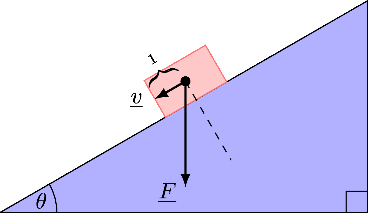
Figure 4.22: The required vector \(\underline{v}\) using the Scalar Product approach.

You just need the vector \(\underline{v}\), with \(\operatorname{length}(\underline{v})=1\), as per Figure 4.22, and then the force’s resolution/projection down the slope is calculated via

\[ \underline{F}\cdot\underline{v}. \]

Note, in this example we haven’t calculated \(\underline{v}\) but in many examples you will already have a vector from previous calculations you can use for \(\underline{v}\) – which you perhaps need to scale first to make it of length \(1\).

Numerical example of Scalar projection

Consider a force \(\underline{F} = \begin{pmatrix}4\\3\end{pmatrix}\), which you can check has magnitude⁶¹ of \(5\) and so represents a force of \(5\) Newtons, and you wish to know how much effect this force has in the Southeast direction\(\ldots\)

We start with a vector which points in the Southeast direction like

\[\underline{u}=\begin{pmatrix}1\\-1\end{pmatrix}.\]

Unfortunately, this vector has length

\[\sqrt{(1)^2+(-1)^2} = \sqrt{2} \neq 1\]

So we divide \(\underline{u}\) by its length to create a new vector which points in the same direction, but is of length \(1\)⁶². So we divide \(\underline{u}\) by \(\sqrt{2}\) via scalar multiplication:

\[ \textrm{Let } \underline{v} = \frac{1}{\sqrt{2}}\times \underline{u} = \begin{pmatrix}\frac{1}{\sqrt{2}}\\-\frac{1}{\sqrt{2}}\end{pmatrix} \approx \begin{pmatrix}0.707\\-0.707\end{pmatrix} \]

This vector \(\underline{v}\) points in the Southeast direction and had length \(1\) so the size of the force \(\underline{F}\) which acts in the Southeast direction is calculated as

\[ \underline{F}\cdot\underline{v} \approx \begin{pmatrix}4\\3\end{pmatrix}\cdot \begin{pmatrix}0.707\\-0.707\end{pmatrix} = 0.707 \textrm{ N}. \]

Notice that the original force \(\underline{F}\) actually had strength of \(5\) N, but not much of it acts in the Southeast direction, only \(0.707\) Newtons worth.

4.11.4 Calculating the “work done” by a force

Another important concept in mechanics is the work done by a force. This quantifies how much energy is transferred by the force during the movement of an object.

It has a formal definition, which is actually very simple.

The definition of work done

If a force \(\underline{F}\) acts upon an object, and results in a displacement vector (from any original position) represented by \(\underline{d}\) then

\[ \textrm{Work done } = \underline{F}\cdot\underline{d}. \]

This says that the Work done is just the Scalar Product of the force acting with the displacement which occurred.

If a number of different forces, \(\underline{F}_1,\underline{F}_2,\underline{F}_3,\ldots\) all act upon an object you can work out individually how much work each force contributed to an overall displacement by separately calculating \(\underline{F}_1\cdot\underline{d}, \underline{F}_2\cdot\underline{d}, \underline{F}_3\cdot\underline{d}, \ldots\). The overall work done is then the sum of these individual answers.

Example

If the wind, represented by a force \(\underline{F}\), moves an object from a location \(P\) to a location \(Q\) then how much work is done by the wind?

We start by calculating the displacement, \(\overrightarrow{PQ}\), see Section 4.8.

Then we calculate

\[ \textrm{Work done } = \underline{F}\cdot \overrightarrow{PQ} \]

For example, if \(\underline{F} = \begin{pmatrix}25\\5\end{pmatrix}\) and the object is moved from point \(P\) with co-ordinates \((1,5)\) to point \(Q\) with co-ordinates \((10,18)\) then the work done is

\[ \begin{pmatrix}25\\5 \end{pmatrix} \cdot \begin{pmatrix}9\\13 \end{pmatrix} = 25\times 9 + 5 \times 13 = 290 \textrm{ (Joules)}. \]

Practice

How much work is done by the force \(\underline{F} = \begin{pmatrix}-2\\3\end{pmatrix}\), in moving an object from location \(P = \left(3 , 1\right)\), to location \(Q = \left(-4 , 3\right)\)?

Answer⁶³

4.12 Vectors in more than 2 dimensions

Two-dimensional (2D) vectors are easy to visualize and also easy to sketch as they can be drawn on a flat piece of paper. Three dimensional vectors, however, require more spatial reasoning skills to visualize, and are harder to draw on 2D surfaces like computer screens.

Here’s an attempt:

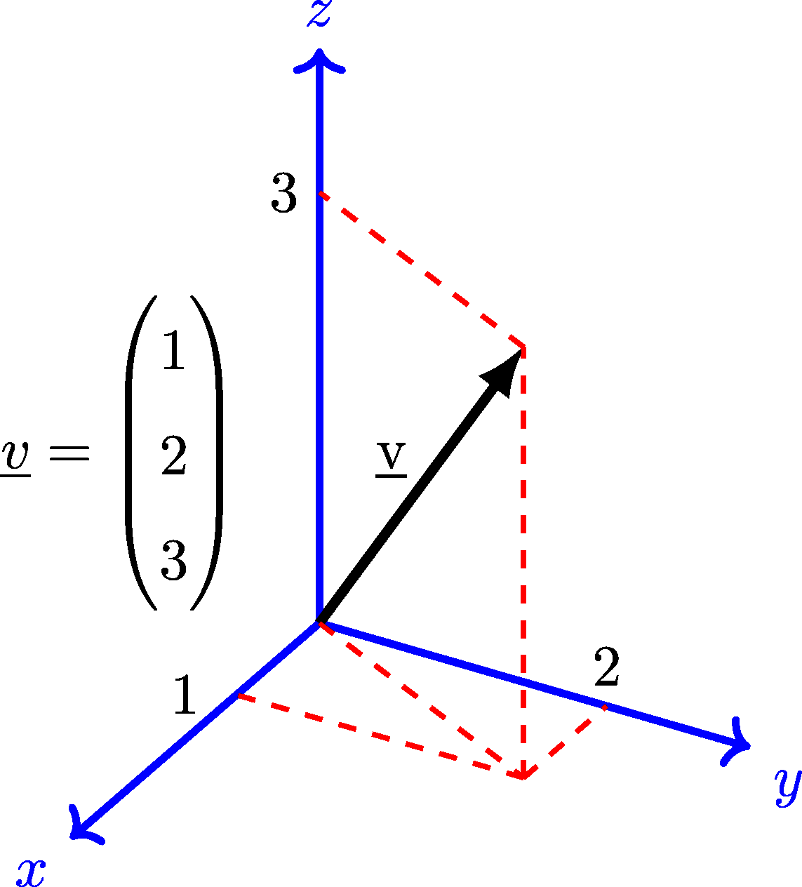
Figure 4.23: An attempt to show a 3D-vector (on a 2D screen).

As you can see the standard rectangular notation matrix format has been extended to just contain a longer column vector like this:

\[ \underline{v} = \begin{pmatrix}1\\2\\3 \end{pmatrix}. \]

Indeed one can generalize this process to as many dimensions as you wish, writing longer and longer vectors, however our human brains aren’t very good at visualizing beyond three dimensions, and there aren’t as many real-world applications to vectors beyond \(3\)-dimensions. We read the first component as the \(x\)-coordinate, then the second component as the \(y\)-coordinate and finally the third component as the \(z\)-coordinate.

In the \(\underline{i},\underline{j}\) notation introduced in Section 4.9, you can just introduce \(\underline{k}=\begin{pmatrix}0\\0\\1\end{pmatrix}\) to represent the third dimension. Extending the existing \(\underline{i}\) and \(\underline{j}\) in the natural way as \(\underline{i}=\begin{pmatrix}1\\0\\0\end{pmatrix}\) and \(\underline{j}=\begin{pmatrix}0\\1\\0\end{pmatrix}\). This vector \(\underline{v}\) can then be written \(\underline{v}=\underline{i}+2\underline{j}+3\underline{k}\).

4.12.1 Adding, subtracting and scaling 3D vectors

The great news is that the rules for performing algebra on vectors in 2D extend completely as expected to 3D vectors.

• Addition and subtraction work the same. You just have a third calculation to do each time. (See equations (4.2) and (4.3))
• Scalar multiplication is the same. You just have to multiple all three components by the scalar. (See equation (4.4))

Examples

\[ \begin{pmatrix} 1\\ 3\\ -4 \end{pmatrix} + \begin{pmatrix} 2 \\ -1 \\ 3 \end{pmatrix} = \begin{pmatrix} 1+2 \\ 3+(-1) \\ (-4)+3 \end{pmatrix} = \begin{pmatrix} 3 \\ 2 \\ -1 \end{pmatrix} \]

and

\[ 3 \times \begin{pmatrix} 1 \\ 0 \\ - 2 \end{pmatrix} = \begin{pmatrix} 3 \\ 0 \\ -6 \end{pmatrix} \]

4.12.2 Lengths for 3D vectors

Amazingly even Pythagoras can be extended to work in more than two dimensions. The standard formula is that you need to calculate the sum of the squares of all the coordinates.

So if \(\underline{v}=\begin{pmatrix}-2 \\ 7 \\ 3\end{pmatrix}\) then \[ \operatorname{length}(\underline{v}) = |\underline{v}| = \sqrt{(-2)^2+7^2+3^2} = \sqrt{62}. \]

4.12.3 Scalar Product for 3D vectors

Even our Scalar Product formula can be extended quite easily to three dimensions. There’s just a third product to add on the end of the calculation, as an extension to our 2D version earlier.

If \(\underline{v}=\begin{pmatrix} x \\ y \\z \end{pmatrix}\) and \(\underline{w}=\begin{pmatrix} a \\ b \\c \end{pmatrix}\) then \[ \underline{v}\cdot\underline{w} = xa+yb+zc. \]

An amazing fact is that the second formula for the Scalar Product (equation (4.6)), i.e.

\[ \underline{v}\cdot\underline{w} = \operatorname{length}(\underline{v})\times \operatorname{length}(\underline{w})\times \cos(\theta) \]

is totally unchanged! The angle between the two vectors is now the angle in 3D space between the two vectors. This means the widest angle visible between them, visible to a viewer who moves around so that both vectors are perpendicular to their vision.

The following properties and facts about Scalar Products still work in 3 dimensions:

• The orthogonality rule, in Section 4.11.2, so a Scalar Product of zero still means two vectors form a right-angle.
• The formula for work done remains the same,
• The formula for scalar projection onto another vector remains the same too.

All these properties still working is why this definition of the (Scalar) Product between two vectors is so useful and powerful in many areas.

Here’s an example of a Scalar Product calculation for two 3-dimensional vectors:

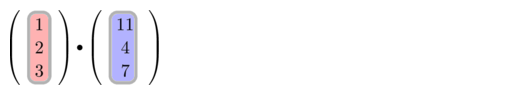
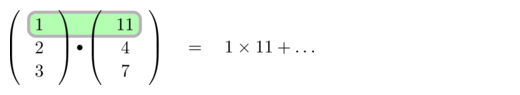
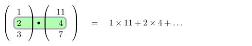
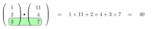
Figure 4.24: Step-by-step Scalar Product calculation of two 3D-vectors.

Let us see how the 3-dimensional Scalar Product can be used to find angles.

Example

A triangle in 3D has vertices⁶⁴ at \(A=(3,2,4)\), \(B=(1,-4,5)\) and \(C=(2,0,-1)\). Determine the angle between the sides \(AB\) and \(AC\).

The angle between the sides \(AB\) and \(AC\) will be the angle between the vectors \(\overrightarrow{AB}\) and \(\overrightarrow{AC}\).

So we begin by finding

\[ \overrightarrow{AB} = \begin{pmatrix} 1-3\\ -4-2\\ 5-4 \end{pmatrix} = \begin{pmatrix} -2\\ -6\\ 1 \end{pmatrix}, \] and \[ \overrightarrow{AC} = \begin{pmatrix} 2-3\\ 0-2\\ -1-4 \end{pmatrix} = \begin{pmatrix} -1\\ -2\\ -5 \end{pmatrix}. \]

To calculate an angle between two vectors we use the Scalar Product formula ((4.6)):

\[ \underline{v}\cdot\underline{w} = \operatorname{length}(\underline{v})\times \operatorname{length}(\underline{w})\times \cos(\theta) \]

In our case, we can easily calculate

\[ \overrightarrow{AB}\cdot\overrightarrow{AC} = 2+12-5 = 9, \]

so re-arranging the Scalar Product formula for the angle \(\theta\) we get

\[ \cos(\theta) = \frac{9}{\operatorname{length}(AB)\operatorname{length}(AC)}. \]

So next we calculate the lengths of our sides, by using (3-dimensional) Pythagoras,

\[ \operatorname{length}(AB) = \sqrt{(-2)^2+(-6)^2+1^2} = \sqrt{41}, \textrm{ and } \] \[ \operatorname{length}(AC) = \sqrt{(-1)^2+(-2)^2+(-5)^2} = \sqrt{30}.\]

So, \(\cos(\theta) = \frac{9}{\sqrt{41}\sqrt{30}} = 0.2566\ldots\). Finally, using \(\cos^{-1}\) we obtain \[ \theta = \cos^{-1}(0.2566\ldots) = 75.13^{\circ}.\]

4.12.4 Polars and other formats for 3D vectors

This is the only topic where 3D vectors become a little messier. You can no longer describe a vector in 3D with just a length and a single angle. Indeed there are competing ways to describe vectors in 3D using at least one angle. We shall not cover them here since they don’t get enormous usage outside of certain specific real-world applications, but an interested reader could go and look them up. The two main formats are:

• Spherical (polar) format, and
• Cylindrical (polar) format.

You will have come across at least one of these before, because the Longitude and Latitude system of co-ordinates for the surface of Planet Earth are actually just Spherical polar co-ordinates where the length is fixed at the Earth’s radius.

4.13 The Vector Product of two vectors

As promised we shall briefly introduce the other invented method for multiplying vectors. This second type of multiplication is called the Vector Product (or the Cross product), it is written with a \(\times\) symbol, e.g. \(\underline{v}\times\underline{w}\).

First two warnings

The Vector Product for vectors is only designed for 3-dimensional vectors.

The Vector Product is messier to calculate than the Scalar Product.

As with the Scalar Product, the name tells you what type of object you get as a result. Let’s see a definition of the Vector Product.

The Vector Product (also called Cross Product) of two vectors, \(\underline{v}\) and \(\underline{w}\) is a calculation written

\[ \underline{v}\times\underline{w}. \]

It is only defined if both \(\underline{v}\) and \(\underline{w}\) are 3-dimensional, e.g.

\[ \underline{v}=\begin{pmatrix} 4\\1\\-5\end{pmatrix} \textrm{ and } \underline{w}=\begin{pmatrix} 2 \\ -9 \\ -3 \end{pmatrix} \]

The general formula is not pretty, and looks like this:

\[\begin{equation} \begin{pmatrix} a\\b\\c \end{pmatrix} \times \begin{pmatrix} d \\ e \\ f \end{pmatrix} = \begin{pmatrix} bf-ce \\ cd-af \\ ae-bd \end{pmatrix} \tag{4.9} \end{equation}\]

Note that unlike the Scalar Product (where the output is a number/scalar), the output of the Vector Product is a vector!

It’s not recommended to try and remember this formula, instead there are a number of different ways to relate this formula to other topics in maths which make it more memorable. Probably the easiest method is via what is known as the determinant of a matrix, which we shall cover in Chapter 5, specifically in Section 5.3.8 and Equation (5.3).

For now we shall just see an example of the calculation, and then make some remarks upon where it is useful.

Taking the sample vectors from above, i.e. \[\begin{equation} \underline{v}=\begin{pmatrix} 4\\1\\-5\end{pmatrix} \textrm{ and } \underline{w}=\begin{pmatrix} 2 \\ -9 \\ -3 \end{pmatrix} \tag{4.10} \end{equation}\]

We can calculate the Vector Product via formula (4.9).

\[\begin{align*} \begin{pmatrix} 4\\1\\-5\end{pmatrix} \times \begin{pmatrix} 2 \\ -9 \\ -3 \end{pmatrix} & = \begin{pmatrix} (1)(-3)-(-5)(-9) \\ (2)(-5)-(4)(-3) \\ (4)(-9)-(1)(2) \end{pmatrix} \\ & = \begin{pmatrix} (-3)-(45) \\ (-10)-(-12) \\ (-36)-(2) \end{pmatrix} \\ & = \begin{pmatrix} -48 \\ 2 \\ -38 \end{pmatrix} \end{align*}\]

Definitely not a pretty calculation, plenty of scope for errors, especially with numerous negative signs.

4.14 Applications of the Vector Product

4.14.1 Finding a “normal” to 2 vectors

The word normal in the context of vectors is an adjective meaning perpendicular to, orthogonal to, or “makes a right-angle with.”

One amazing property⁶⁵ of the Vector Product is that

\[ \underline{v}\times\underline{w} \textrm{ is always perpendicular to both \(\underline{v}\) and \(\underline{w}\)}. \]

So to find a vector which is normal to two other vectors you can just calculate their Vector Product. If you think about it geometrically, in 3-dimensions the answer to this question is unique excepting scalar multiples of the answer. That is, if \(\underline{n}\) is normal to \(\underline{v}\) and \(\underline{w}\) then the only other vectors which are also normal to \(\underline{v}\) and \(\underline{w}\) are vectors that look like \(k\underline{n}\) for all constant values of \(k\).

Let us check this orthogonality claim for \(\underline{v}\times\underline{w}\) for an example, by using our orthogonal property from the Scalar Product we saw in Section 4.11.2.

We can check this with our example we used above to calculate a Vector Product. We begin with \[ \underline{n} = \begin{pmatrix} -48 \\ 2 \\ -38 \end{pmatrix} \] and let us first calculate \(\underline{n}\cdot\underline{v}\) where \(\underline{v}\) and \(\underline{w}\) were defined as \[ \underline{v}=\begin{pmatrix} 4\\1\\-5\end{pmatrix} \textrm{ and } \underline{w}=\begin{pmatrix} 2 \\ -9 \\ -3 \end{pmatrix}. \]

\[\begin{align*} \underline{n}\cdot\underline{v} & = \begin{pmatrix} -48 \\ 2 \\ -38 \end{pmatrix} \cdot \begin{pmatrix} 4\\1\\-5\end{pmatrix} \\ & = -48\times 4+2\times 1+(-38)\times(-5) \\ & = -192+2+190 = 0~~\checkmark \end{align*}\] The Scalar Product was zero, so the two vectors are indeed perpendicular⁶⁶ in 3D.

The second calculation, verifying that \(\underline{n}\cdot\underline{w}=0\) is left for you as an exercise.

4.14.2 Calculating the moment of a force

The moment of a force, also called a torque, is a physics concept representing the turning force around some location. Since these notes are focussed upon the mathematical elements we shall just provide a definition here and not go into the physics.

Definition of moment

If we have a force, \(\underline{F}\), which acts through a point in space we call \(B\), then the moment of this force about another point \(A\) is defined as

\[ \overrightarrow{AB}\times\underline{F}. \]

Recall the notation \(\overrightarrow{AB}\) means the vector joining the point \(A\) to the point \(B\), see Section 4.8.

4.14.3 Other uses of the Vector Product

There are a few other more obscure uses of the Vector Product, they are not worth discussing here, but an interested reader could go and look up shearing force and the volume of a parallelepiped!

4.15 Further practice exercises

There are many more vectors examples for you try, especially for these latter topics, in the specific further exercises Section 7.

As with the algebra chapter, reinforcing your learning is best done by trying examples, so you are recommended to seek out your own further exercises too.

4.16 Summary of chapter

Having worked through this chapter and attempted the exercises you should now have developed understanding of the following topics:

• know what vectors (and scalars) are and identify common notations for them;
• use Cartesian/Rectangular or Polar notations for vectors and be able to convert between them;
• perform basic algebra like addition and scalar multiplication of vectors;
• use vectors to represent relative positions of objects;
• define, calculate and use the Scalar Product of two vectors in various applications;
• define, calculate and use the Vector Product of two three-dimensional vectors in various applications.